Where am I? Project Writeup
Abstract
The second project in term 2 of the Udacity Robotics Nano Degree program requires students to complete a hijacked robot scenario using ROS and Gazebo.
Students are to initially follow instructions for a building a reference robot model, before tuning the localisation parameters satisfactorily such that the robot within the Gazebo maze simulation can reach an end goal.
After completion of that, a new robot model is created with alterations to the base and position of sensors. Whereby it uses the same simulation and must reach the same end goal.
Introduction
In this project a robot model has to use localisation to work out where it is. It creates a rolling local map using laser range sensors. The local map in turn is used to navigate towards a navigation goal.
The navigation stack utilised move_base. It provides a local cost map, as the robot moves, in relation to a global cost map to define a continuous path for the robot to move along.
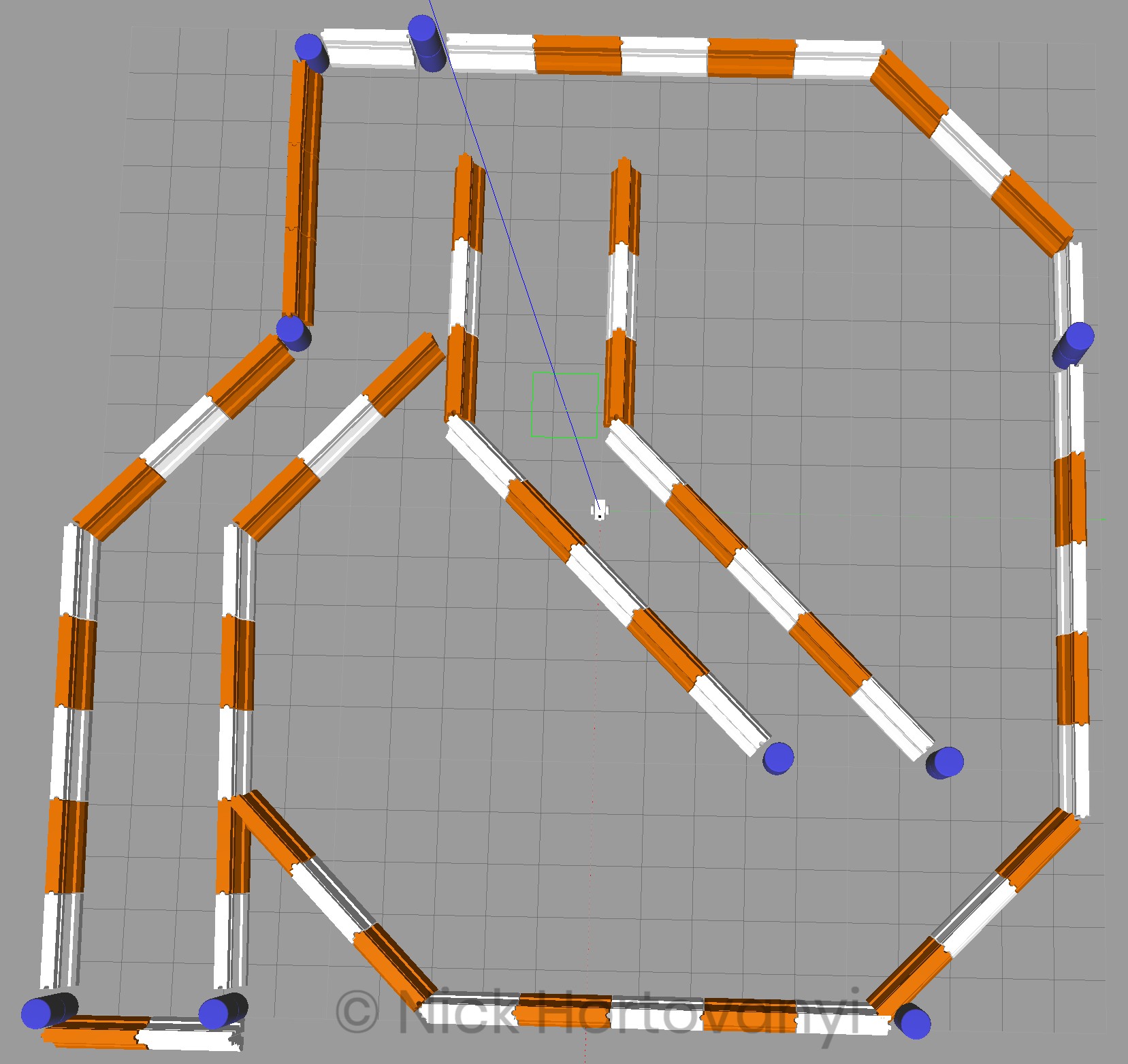
This project utilises Gazebo to create a simulation with a map provided by Clearpath Robotics
Once the robot has reached the navigation goal, the objective of the project has been achieved.
Background
A robot needs to understand where it is in a world, to be able to make navigation plans to get from point a, to point b, whilst avoiding obstacles. The process of understanding “where am I?” (from a robots perspective) is called localisation.
This project uses a localisation package built into ROS called Adaptive Monte Carlo Localisation (AMCL) to assist with the robot in a scenario to work out where it is. Hence the project name “Where am I?”.
AMCL is a variant of the Monte Carlo Localisation (MCL) which was learnt in the course material. MCL uses particles to localise the robot pose. It has several advantages over using Extended Kalman Filters (EKF) such as uses raw measurements (ie from lasers), is not reliant on gaussian noise, is memory and time efficient, and can perform global localisation.
The AMCL package adaptively alters the number of particles used, which has the advantage of reducing the computational overhead required.
Results
We first completed this exercise using the class room example which is named udacity_bot. Then a different version was created where the base and sensor locations were changed. This was named nick_bot and was launched using udacity_world_nick.launch.
The final results of when it reached the goal state follow.
udacity_bot

nick_bot

Model Configuration
This discussion is for the configuration of nick_bot.
The nick_bot was a square version of the rectangle based udacity_bot. The laser sensor was moved to the front of the robot.
The amcl_nick.lauch. Wherever possible the same configuration and parameters as the udacity_bot used amcl.launch.
min_particles was set to 25 and max_particles to 200 to not heavily utilise CPU. A higher max_particles did not improve initial ability of the robot to find itself with certainty.
odom_alpha1 to odom_alpha4 were trial & error values and changed from the default of 0.2 (there was not much documentation about).
The laser model parameters were left as default. There appeared no reason to change them as they were clearly visible on the above rviz visualisations and aligned to the barriers.
The yaw_goal_tolerance and xy_goal_tolerance were doubled from the default values to allow for additional flexibility in trajectory planning.
costmap_common_params_nick.yaml
transform_tolerance was set 1.25 and update_frequency to 3.0 for both local and global.
obstacle_range was set to 1.5, raytrace_range to 4.0 and inflation_radius to 0.65 to enable sufficient space on the cost map for the robot to navigate.
robot_radius was set to 0.4 in this model to allow for the larger square design.
local_costmap_params.yaml
The local publish_frequency was set to 3.0 with the global to 5.0 This configuration in conjunction with 15.0 x 15.0 sized local cost map was able to function within the performance constraints of the system used. Increasing the size of the local cost map utilise significant more computer power and missed the time windows for publish_frequency.
global_costmap_params.yaml
the update and publish frequency were set per above. In addition the width and height were set to the map size.
base_local_planner_params.yaml
sim_time was set to 4 as there appeared sufficient compute resource to estimate a trajectory out 4 seconds.
meter_scoring was enabled to ensure pdist_scale used meters.
pdist_scale was set to 0.5 being less than the default of 0.6. Default and higher values appeared to cause the robot to sometimes get stuck.
Discussion
The robot model was able to on most runs navigate successfully to the goal. The route taken at times could have been shortened. However further research is required into the ROS packages used to be able to tune it to achieve such. Often the observed path taken did not appear to be the most cost affective and when it missed the target goal, it would do a large sweep before re-approaching the target.
The AMCL routine appeared to quickly gain certainty about the locality of the robot. It was the rest of the navigation stack and move_base that needed further tuning.
In the kidnapped robot problem where by a robot is positioned in an arbitrary location, AMCL would be able to adapt the number of particles used to gain certainty of the robot’s location. In addition AMCL does not rely on landmarks, but on laser based maps, laser scans and transform messages to output pose estimates.
Moreover in an environment, where by there weren’t known landmarks, the AMCL has advantages over the Extended or Unscented Kalman Filter based approaches. These environments would include those with no known map (ie its the first time being navigated) or in highly unstructured environments with lots of moving structures over time eg shopping centres with popup shops in the aisles with significant foot traffic.
Future Work
The size of the local cost map had a significant impact on performance. Higher values decreased the ability to publish within the frequency required. In addition higher particle numbers whilst increasing CPU load did not reduce the time taken for the AMCL to be certain about the robots locality.
A square designed robot model as opposed to a rectangular design appeared to enable the robot to rotate more affectively around its base. Other wheel components are available but they did not publish ODOM information. Hence additional sensors might be required with further investigation into the impact of the removal of ODOM readings required.
A laser GPU gazebo component was available. This may enable reduced CPU load by moving the workload to the GPU.
A LIDAR unit would give a more complete map of the world around the robot. One could also look to include more laser sensors to map behind and to either side of the robot. This should facilitate with the creation of a more complete motion plan without the need for the robot to map it first.
When implementing this type of project on real hardware, the mobile nature of a robot, requiring it also to contain its own power sources, means that efficient usage of a CPU and GPU are a must. The higher the utilisation, the less effective time the robot will have to perform activities.
Thus whilst implementing more sensors may provide a more detailed and accurate map, in the field this would further drain the power source. Hence careful consideration is needed for the number of sensors, the total power consumption of the sensors and compute work loads, as well as the impact the quantity of data has to the compute utilisation rates whilst mobile.
If there no significant improvement in performance for the design objective and operational goals of the robot, then a more minimalist sensor and localisation cost map configuration may be appropriate.

