Advanced Lane Detection

In this Advanced Lane Detection project, we apply computer vision techniques to augment video output with a detected road lane, road radius curvature and road centre offset. The video was supplied by Udacity and captured using the middle camera.

sample lane detection result

The goals / steps of this project are the following:

• Compute the camera calibration matrix and distortion coefficients given a set of chessboard images.
• Apply a distortion correction to raw images.
• Use color transforms, gradients, etc., to create a thresholded binary image.
• Apply a perspective transform to rectify binary image (“birds-eye view”).
• Detect lane pixels and fit to find the lane boundary.
• Determine the curvature of the lane and vehicle position with respect to center.
• Warp the detected lane boundaries back onto the original image.
• Output visual display of the lane boundaries and numerical estimation of lane curvature and vehicle position.

A jupyter/iPython data science notebook was used and can be found on github Full Project Repo – Advanced Lane Finding Project Notebook (Note the interactive ipywidgets are not functional on github). The project is written in python and utilises numpy and OpenCV.

Camera Calibration

Every camera has some distortion factor in its lens. The known approach to correct for that in (x,y,z) space is apply coefficients to undistort the image. To calculate this a camera calibration process is required.

It involves reading a set of warped chessboard images, converting them into grey scale images before using cv2.findChessboardCorners() to identify the corners as imgpoints.

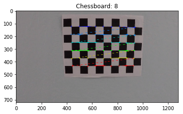
If corners are detected then they are collected as image points imgpoints along with a set of object points objpoints; with an assumption made that the chessboard is fixed on the (x,y) plane at z=0 (object points will hence be the same for each calibration image).

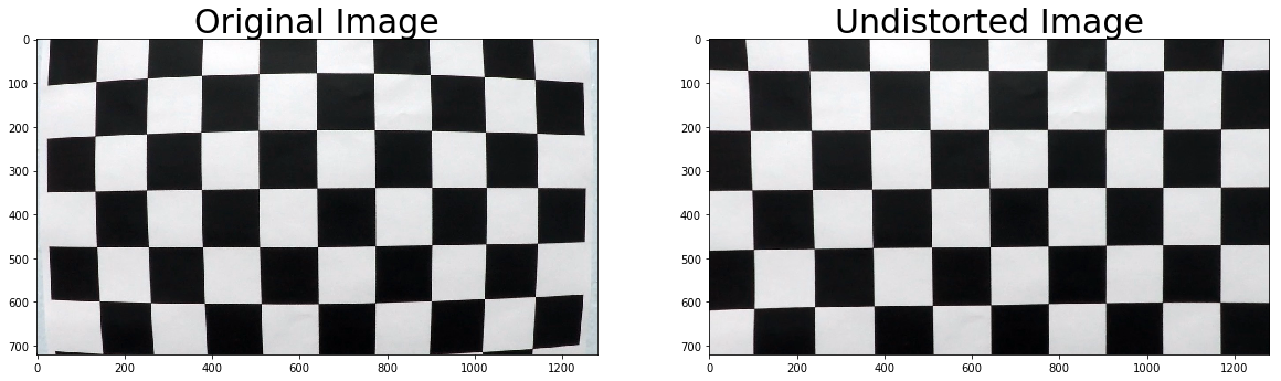
In the function camera_calibrate I pass the collected objpoints, imgpoints and a test image for the camera image dimensions. It in turn uses cv2.calibrateCamera() to calculate the distortion coefficients before the test image is undistorted with cv2.undistort() giving the following result.

Pipeline (Test images)

After camera calibration a set of functions have been created to work on test images before later being used in a video pipeline.

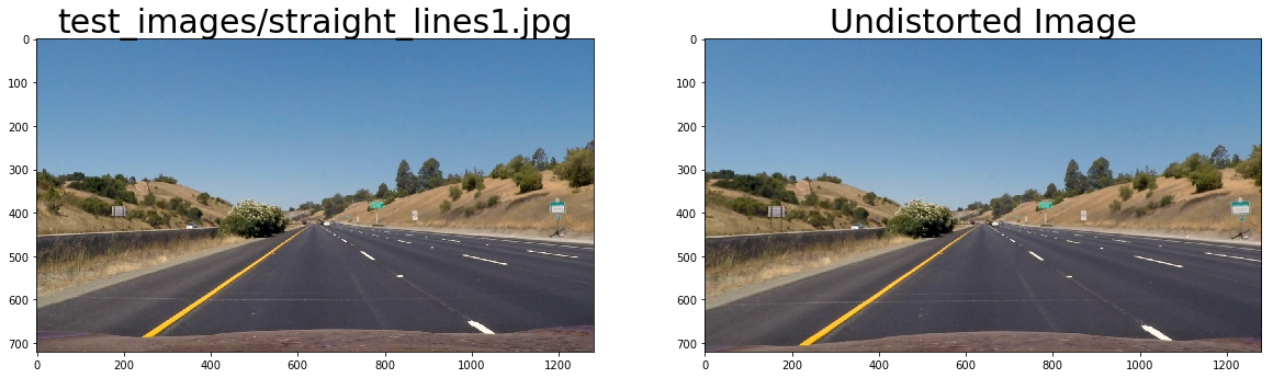
Distortion corrected image

The undistort_image takes an image and defaults the mtx and dist variables from the previous camera calibration before returning the undistorted image.

Threshold binary images

A threshold binary image, as the name infers, contains a representation of the original image but in binary 0,1 as opposed to a BGR (Blue, Green, Red) colour spectrum. The threshold part means that say the Red colour channel( with a range of 0-255) was between a threshold value range of 170-255, that it would be set to 1.

A sample output follows.

Initial experimentation occurred in a separate notebook before being refactored back into the project notebook in the combined_threshold function. It has a number of default thresholds for sobel gradient x&y, sobel magnitude, sober direction, Saturation (from HLS), Red (from RGB) and Y (luminance from YUV) plus a threshold type parameter (daytime-normal, daytime-bright, daytime-shadow, daytime-filter-pavement).

Whilst the daytime-normal threshold worked great for the majority of images there were situations where it didn’t e.g. pavement colour changes in bright light and shadow.

Daytime Normal with noise bright light & pavement change

Daytime Normal with shadow

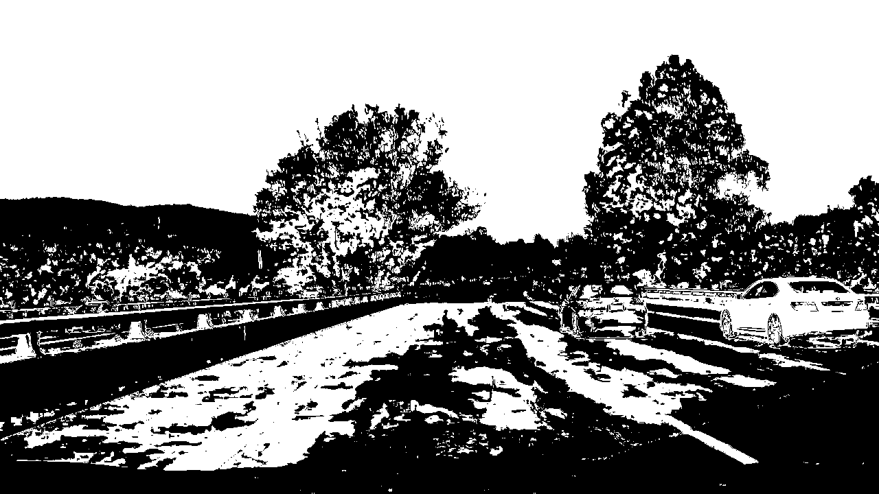
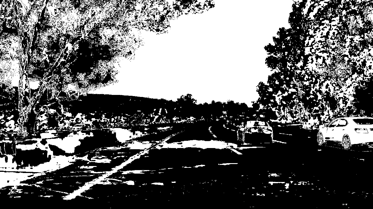
Other samples Daytime Bright, Daytime Shadow and Daytime Filter Pavement.

Perspective transform – birds eye view

To be able to detect the road lines, the undistorted image is warped. The function calc_warp_points takes an image’s height & width and then calculates the src and dst array of points. perspective_transforms takes them and returns two matrixes M and Minv for perspective_warp and perpective_unwarp functions respectively. The following image, shows an undistorted image, with the src points drawn with the corresponding warped image (the goal here was straight lines)

Lane-line pixel identification and polynomial fit

Once we have a birds eye view with a combined threshold we are in a position to identify lines and a polynomial to draw a line (or to search for points in a binary image).

topdown warped binary image

A histogram is created via lane_histogram from the bottom third of the topdown warped binary image. Within lane_peaks, scipy.signal is used to identify left and right peaks. If just one peak then the max bin either side of centre is returned.

calc_lane_windows uses these peaks along with a binary image to initialise a left and right instance of a WindowBox class. find_lane_window then controls the WindowBox search up the image to return an array of WindowBoxes that should contain the lane line. calc_fit_from_boxes returns a polynomial or None if nothing found.

poly_fitx function takes a fity where
fity = np.linspace(0, height-1, height) and a polynomial to calculate an array of x values.

The search result is plotted on the bottom left of the below image with each box in green. To test line searching by polynomial, I then use the left & right WindowBox search polynomials as input to calc_lr_fit_from_polys. The bottom right graphic has the new polynomial line draw with a blue search window (relates to polynomial used for the search from WindBoxes) that was used overlapping with a green window for the new.

Warped box seek and new polynomial fit

Radius of curvature calculation and vehicle from centre offset

In road design, curvature is important and its normally measured by its radius length. For a straight line road, that value can be quite high.

In this project our images are in pixel space and need to be converted into meters. The images are of US roads and I measured from this image the distance between lines (413 pix) and the height of dashes (275 px). Lane width in the US is ~ 3.7 meters and dashed lines 3 metres. Thus xm_per_pix = 3.7/413 and ym_per_pix = 3./275 were used in calc_curvature. The function converted the polynomial from pixel space into a polynomial in meters.

To calculate the offset from centre, I first determined where on the x plane, both the left lx and right rx lines crossed the image near the driver. I then calculated the xcentre of the image as the width/2. The offset was calculated such (rx - xcenter) - (xcenter - lx) before being multiple by xm_per_pix.

Final pipeline

I decided to take a more python class based approach once I progressed through this project. Inside the classes, I called the functions mentioned previously. The classes created were:

• Lane contains image processing, final calculations for view drawing and reference to left and right RoadLines. It also handled searching for initial lines, recalculations and reprocessing a line that was not sane;
• RoadLine contains a history of Lines and associated curvature and plotting calculations using weighted means; and
• Line contains detailed about the line and helper functions

Processing is triggered by setting the Lane.image variable. Convenient property methods Lane.warped, Lane.warped_decorated, lane.result and lane.result_decorated return processed images. It made it very easy to debug output using interactive ipywidgets (which don’t work on github)

Sample result images

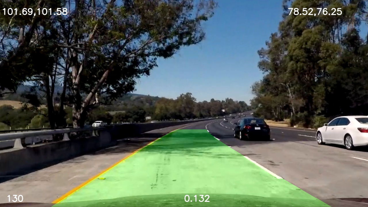
lane.result_decorated

Lane.warped_decorated

Pipeline (Video)

Using moviepy to process the project video was simple. I also decorated the result with a frame count. The Project Video Lane mp4 on GitHub, contains the result (YouTube Copy)

Discussion

Problems/Issues faced

To some degree, I got distracted with trying to solve the issues I found in my algorithm with the challenge videos. This highlighted, that I need to improve my understanding of colour spaces, sobel and threshold combinations.

I included a basic algorithm to remove pavement colours from the images using a centre, left and right focal point. I noticed that the dust colour on the vehicle seemed to be also in the road side foliage. This however wasn’t sufficient to remove all pavement colour and didn’t work when there was a road type transition. It was very CPU intensive.

In the end, I used a combination of different methods, that used a basic noise filter on warped binary images to determine, if it was sufficient to look for a line or not. If it wasn’t it tried the next one, with the final being a vertical rectangle window crawl down the image. Where the best filter was determined for each box. Again this was CPU intensive, but worked.

Another issue faced was using the previous curvature radius to determine if this line was sane or not. The values were too jittery and when driving on a straight line, high. I decided not to pursue this.

Opportunities for improvement in the algorithm/pipeline

There is room here for some refactoring into a more Object oriented approach. This was not evident at the start of the project as to how it should be structured. I experimented a little with using Pool from multiprocessing to parallelise left and right lane searches. It didn’t make it into my final classes as for normal line searching using a polynomial, as I did not ascertain if the multiprocessing overhead, outweighed the parallelism value. Certainly potential here to use a more functional approach to give the best runtime options for parallelisation.

Other areas, include automatically detecting the src points for warp, handling bounce in the road and understanding surface height (above road) of the camera and its impact.

I thought also as I’ve kept history, I could extend the warp to include a bird’e eye representation of the car on the road and directly behind it. I did mean averaging on results for smoothing drawn lines, but this was not included in the new line calculations from the next image frames.

The algorithm could also be made to make predictions about the line when there is gaps. This would be easier with continuous lines then dashed.

Hypothetical pipeline failure cases

Pavement fixes and/or combined with other surfaces that create vertical lines near existing road lines.

It would also fail if there was a road crossing or a need to cross lanes or to exit the freeway.

Rain and snow would also have an impact and I’m not sure about night time.

Tail gating a car or a car on a tighter curve would potentially interrupt the visible camera and hence line detection.

Clone Driving Behaviour

Clone driving behaviour using Deep Learning

With this behaviour cloning project, we give steering & throttle instruction to a vehicle in a simulator based on receiving a centre camera image and telemetry data. The steering angle data is a prediction for a neural network model trained against data saved from track runs I performed.

The training of the neural net model, is achieved with driving behaviour data captured, in training mode, within the simulator itself. Additional preprocessing occurs as part of batch generation of data for the neural net training.

Model Architecture

I decided to as closely as possible use the Nvidia’s End to End Learning for Self-Driving Cars model. I diverged by passing cropped camera images as RGB, and not YUV, with adjusting brightness and by using the steering angle as is. I experimented with using 1/r (inverse turning radius) as input but found the values were too small (I also did not know the steering ratio and wheel base of the vehicle in the simulator).

Additional experimentation occurred with using comma.ai, Steering angle prediction model but the number of parameters was higher then the nvidia model and it worked off of full sized camera images. As training time was significantly higher, and initial iterations created an interesting off road driving experience in the simulator, I discontinued these endeavours.

The model represented here is my implementation of the nvidia model mentioned previously. It is coded in python using keras (with tensor flow) in model.py and returned from the build_nvidia_model method. The complete project is on github here Udacity Behaviour Cloning Project

Input

The input is 66x200xC with C = 3 RGB color channels.

Architecture

Layer 0: Normalisation to range -1, 1 (1./127.5 -1)

Layer 1: Convolution with strides=(2,2), valid padding, kernel 5×5 and output shape 31x98x24, with elu activation and dropout

Layer 2: Convolution with strides=(2,2), valid padding, kernel 5×5 and output shape 14x47x36, with elu activation and dropout

Layer 3: Convolution with strides=(2,2), valid padding, kernel 5×5 and output shape 5x22x48, with elu activation and dropout

Layer 4: Convolution with strides=(1,1), valid padding, kernel 3×3 and output shape 3x20x64, with elu activation and dropout

Layer 5: Convolution with strides=(1,1), valid padding, kernel 3×3 and output shape 1x18x64, with elu activation and dropout

flatten 1152 output

Layer 6: Fully Connected with 100 outputs and dropout

Layer 7: Fully Connected with 50 outputs and dropout

Layer 8: Fully Connected with 10 outputs and dropout

dropout was set aggressively on each layer at .25 to avoid overtraining

Output

Layer Fully Connected with 1 output value for the steering angle.

Visualisation

Keras output plot (not the nicest visuals)

Data preprocessing and Augmentation

The simulator captures data into a csv log file which references left, centre and right captured images within a sub directory. Telemetry data for steering, throttle, brake and speed is also contained in the log. Only steering was used in this project.

My initial investigation and analysis was performed in a Jupyter Notebook here.

Before being fed into the model, the images are cropped to 66×200 starting at height 60 with width centered – A sample video of a run cropped.

Cropped left, centre and right camera image

As seen in the following histogram a significant proportion of the data is for driving straight and its lopsided to left turns (being a negative steering angle is left) when using data generated following my conservative driving laps.

The log file was preprocessed to remove contiguous rows with a history of >5 records, with a 0.0 steering angle. This was the only preprocessing done outside of the batch generators used in training (random rows are augmented/jittered for each batch at model training time).

A left, centre or right camera was selected randomly for each row, with .25 angle ( for left and – for right) applied to the steering.

Jittering was applied per Vivek Yadav’s post to augment data. Images were randomly transformed in the x range by 100 pixels and in the y range by 10 pixels with 0.4 per xpixel adjusted against the steering angle. Brightness via a HSV (V channel) transform (.25 a random number in range 0 to 1) was also performed.

During batch generation, to compensate for the left turning, 50% of images were flipped (including reversing steering angle) if the absolute steering angle was > .1.

Finally images are cropped per above before being batched.

Model Training

Data was captured from the simulator. I drove conservatively around the track three times paying particular attention to the sharp right turn. I found connecting a PS3 controller allowed finer control then using the keyboard. At least once I waited till the last moment before taking the turn. This seems to have stopped the car ending up in the lake. Its also helped to overcome a symptom of the bias in the training data towards left turns. To further offset this risk, I validated the training using a test set I’d captured from the second track, which is a lot more windy.

Training sample captured of left, centre and right cameras cropped

Center camera has the steering angle and 1/r values displayed.

Validation sample captured of left, centre and right cameras cropped

Center camera has the steering angle and 1/r values displayed.

The Adam Optimizer was used with a mean squared error loss. A number of hyper-parameters were passed on the command line. The command I used looks such for a batch size of 500, 10 epochs (dropped out early if loss wasn’t improving), dropout at .25 with a training size of 50000 randomly augmented features with adjusted labels and 2000 random features & labels used for validation

python model.py --batch_size=500 --training_log_path=./data --validation_log_path=./datat2 --epochs 10 \
--training_size 50000 --validation_size 2000 --dropout .25

Model Testing

To meet requirements, and hence pass the assignment, the vehicle has to drive around the first track staying on the road and not going up on the curb.

The model trained (which is saved), is used again in testing. The simulator feeds you the centre camera image, along with steering and throttle telemetry. In response you have to return the new steering angle and throttle values. I hard coded the throttle to .35. The image was cropped, the same as for training, then fed into the model for prediction giving the steering angle.

steering_angle = float(model.predict(transformed_image_array, batch_size=1))
throttle = 0.35

Successful run track 1

Successful run track 2

note: the trained model I used for the track 1 run, is different to the one used to run the simulator in track 2. I found that the data I originally used to train a model to run both tracks, would occasionally meander on track 1 quite wildly. Thus used training data to make it more conservative to meet requirements for the projects.

My first lane detection algo

I’m all for practical learning by building things. There’s nothing like getting stuck into a project and seeing results. Whilst a little progress is a good motivator, it also shows you how much it is that you don’t know.

I was pleased with the results of my first project doing the Udacity Self Driving Car Engineer Nanodegree. Yet what was more pleasing was being shown how much experimentation is really required. That is that is so much to learn.

This first module was about understanding some of the principles of computer vision that apply. We first started with Canny Edge Detection

and then Hough transform to detect lines within a region of interest.

The first project was to apply this learning, first to set of static images and then to a couple of videos captured whilst driving on a highway.

How cool is the final result .

I submitted my Jupyter Notebook for review. To pass you need to ensure that you meet specification. I passed here is the review feedback.

Some of my reflection thoughts on what can be improved in a future iteration of the project:

• look for the road horizon starting from bottom centre of the image working up – asphalt has a fairly unique colour
• break ROI into left and right lanes earlier – seems that at least with driving on a highway without lane changing that we can assume with confidence where they should start at the base of the image
• segment each ROI into chained vertical blocks of a smaller width
• when drawing connect intersection of cv2.fitLine lines
• increase number of segments if lanes are curving left or right
• label the lines with colour and type – continuous, dashed etc
• feed the previous result into the evaluation of the next image
• determine when an image has no lanes that could be considered reasonable
• lane changing and entering a lane from a curb needs more though
• if using smaller more specific left and right lane ROIs should allow for following a vehicle
• not sure how rain affects this – might have to do a test and capture video in a tropical down pour this storm season
• this approach wouldn’t work in snow. would require a different approach

Its still early yet in the nano degree but I’m hooked already. Happy coding and driving.

Congratulations – You’ve been Accepted

It was my birthday and a little email arrived from Udacity titled “Congratulations, you’re going to be one of our very first Self-Driving Car students!”. I had never thought with the number of people that were applying that I’d have a chance. Yet here was the email as a birthday present. I was both thrilled and apprehensive – I’d gotten in and now had to follow through.

I’ve been fascinated with robotics and AI for quite sometime now. And as always I seem to be too early with investigating business endeavours in Australia related to such. Whilst my cycling project was interesting, I was getting bogged down with having to learn how to use all the technology by myself. It always surprised me that I was able to get some results given how large the US teams seems to be that were using the same open source projects.

I’d applied to the program, because I thought I could leverage what I’d been learning through my previous endeavours around learnings from my cycling big data sensor project. The course had a focus on using things like ROS (Robotic Operating System), TensorFlow and Open Computer Vision. Plus it’d just seemed to be a great idea to work on technology related to self driving vehicles in a structured way. There is so much interest in this subject matter.

When I shared with my Facebook friends, that I’d been accepted, it was the most liked post I think I’ve ever had. Speaking people they say “wow thats great”. So its past the litmus test and I’ve just started.