Vehicle Detection and Tracking

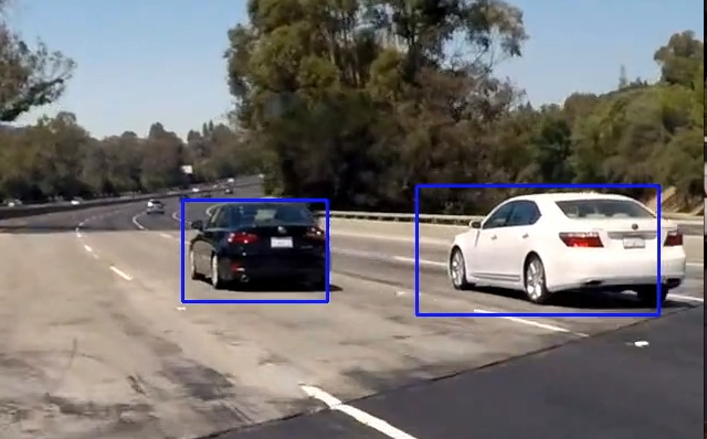
In this vehicle detection and tracking project, we detect in a video pipeline, potential boxes, via a sliding window, that may contain a vehicle by using a Support Vector Machine Classifier for prediction to create a heat map. The heat map history is then used to filter out false positives before identification of vehicles by drawing a bounding box around it.

Vehicle Detection Sample

Vehicle Detection Project

The goals / steps of this project are the following:

  • Perform a Histogram of Oriented Gradients (HOG) feature extraction on a labeled training set of images and train a classifier Linear SVM classifier
  • Optionally, you can also apply a color transform and append binned color features, as well as histograms of color, to your HOG feature vector.
  • Note: for those first two steps don’t forget to normalize your features and randomize a selection for training and testing.
  • Implement a sliding-window technique and use your trained classifier to search for vehicles in images.
  • Run your pipeline on a video stream (start with the test_video.mp4 and later implement on full project_video.mp4) and create a heat map of recurring detections frame by frame to reject outliers and follow detected vehicles.
  • Estimate a bounding box for vehicles detected.

A jupyter/iPython data science notebook was used and can be found on github Full Project RepoVehicle Detection Project Notebook (Note the interactive ipywidgets are not functional on github). As the notebook got rather large I extracted some code into python files utils.py (functions to extract, loading helpers), features.py (feature extraction and classes), images.py (image and window slice processing), search.py (holds search parameters class), boxes.py (windowing and box classes) and detection.py (main VehicleDetection class that coordinates processing of images). The project is written in python and utilises numpy, OpenCV, scikit learn and MoviePy.

Histogram of Oriented Gradients (HOG)

Through a bit of trial and error I found a set of HOG parameters.

HOG Feature Extraction and Parameters

A function extract_hog_features was created that took an array of 64x64x3 images and returned a set of features. These are extracted in parallel and it in turn uses HogImageFeatures class.

As the hog algorithm is primarily focused on grey images, I initially used the YCrCB colour space with the Y channel (used to represent a gray images). However I found that it was not selective enough during the detection phase. I thus used all 3 colour channels. To reduce the number of features, I increased the number of HOG pixels per cell. I used an interactive feature in my notebook to find an orient setting of 32 that showed distinctive features of vehicle. Sample follows.

Training Vehicle HOG Sample

The final parameter settings used color_space = 'YCrCb',orient = 32,pix_per_cell = 16 and hog_channel = 'ALL'. Experimentation occurred with using Colour Histogram Features but it slowed down feature extraction and later increased the number of false positives detected. Per the following visualisation graphic, you can see that the Cr and Cb colour spaces had detectable hog features

Sample HOG Channel Output form a video window slice

Classifier Training

Once HOG features (no Colour Hist or Bin Spatial) were extracted from car (GTI Vehicle Image Database and Udacity Extras) and not_car (GTI, KITTI) image sets. They were then stacked and converted to float in the vehicle detection notebook.

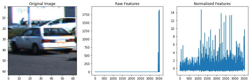
Features were then scaled using the Sklearn RobustScaler sample result follows.
RobustScaler Feature Sample

Experimentation occurred in the Classifier Experimentation Notebook between LinearSVC (Support Vector Machine Classifier), RandomForest and ExtraTrees classifiers. LinearSVC was chosen as the prediction time was 0.00228 seconds for 10 labels compared to ~0.10 seconds for the other two.

Sliding Window Search

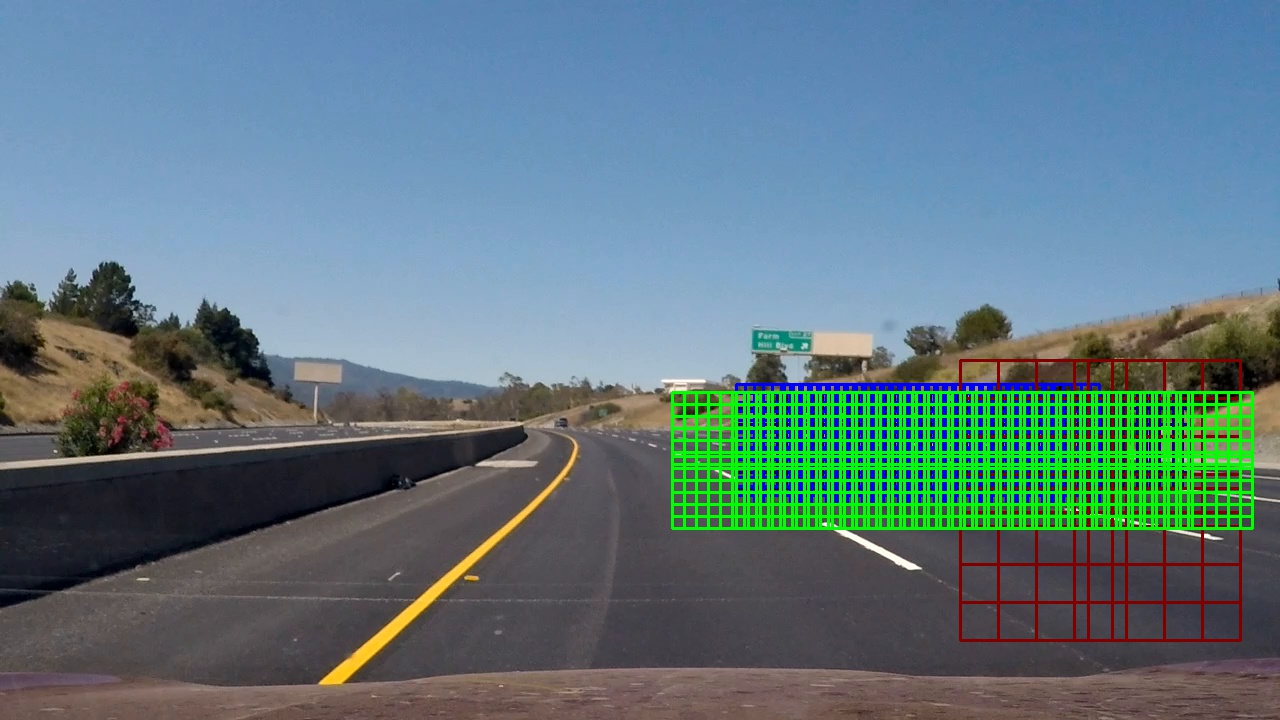
Building sliding windows

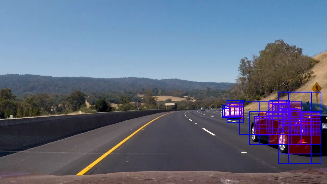
For this project four sizes of windows were chosen – 32×32, 48×48, 64×64 and 128×128 and position at different depth perspective on the bottom right side of the image to cover the road. The larger windows closer to the driver and the smaller closer to the horizon. Overlap in both x,y was set between 0.5 and 0.8 to balance the need for better coverage vs number of boxes generated – currently 937. The more boxes for a sliding window, the more calculations per video image.
Window Search Example

Classifier examples and optimisation

Some time was spent on parallelisation of the search using Python async methods and asyncio.gather in the VehicleDetection class. The search extracts the bounded box image of each sized search window and scales it to 64×64 before doing feature extraction and prediction on each window.
Small Window Slice Scaled to 64x64

The search hot_box_search returns an array of hot boxes that classifier has predicted contains a vehicle.

These boxes overlap and are used to create a clipped at 255, two dimensional heat map. To remove initial false positives counts > 4 are kept. The heat map is then normalised before another threshold is applied

heatmap = apply_threshold(heatmap, 4)
heatmap_std = heatmap.std(ddof=1)
if heatmap_std != 0.0:
    heatmap = (heatmap-heatmap.mean())/heatmap_std
heatmap = apply_threshold(heatmap, np.max([heatmap.std(), 1]))    

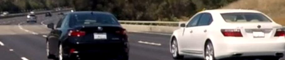
Plotting this stage back onto the image
detected boxes and heatmap

A history is kept of heat maps Heatmap History which is then used as input into Scipy Label with a dim binary structure linking dimensions, giving
Heatmap with corresponding 2 cars identified labels
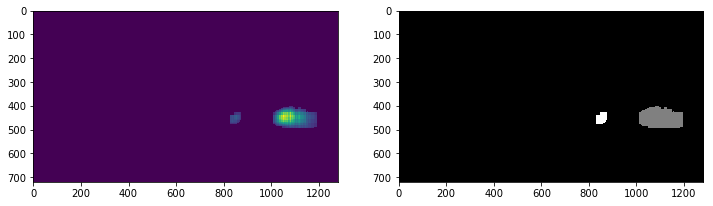
finally a variance filter is applied on each box, if for one detected label boxes are ignored with a variance < 0.1 (its just a few close points0 or if multiple with a variance < 1.5 (more noise).

Video Implementation

Vehicle Detection Video

The Project VehicleDetection mp4 on GitHub, contains the result (YouTube Copy)

Result Video embedded from YouTube

Tracking Vehicle Detections

One of the nice features of the scipy.ndimage.measurements.label function is that it can process 3d arrays giving labels in x,y,z spaces. Thus when using the array of heat map history as input, it labels connections in x,y,z. If a returned label box is not represented in at least 3 (heat map history max – 2) z planes then it is rejected as a false positive. The result is that a vehicle is tracked over the heat map history kept.

Discussion

When construction this pipeline, I spent some time working on parallelising the window search. What I found is that there is most likely little overall performance improvement to be gained by doing so. Images have to be processed in series and whilst generating the video, my cpu was under utilised.

In hindsight I should of used a heavy weight search to detect vehicles and then a more lighter weight, narrower search primed by the last known positions. Heavy weight searching could be run at larger intervals or when a vehicle detection is lost.

My pipeline would fail presently if vehicles were on the left hand side or centre of the car. I suspect trucks, motorbikes, cyclists and pedestrians would not be detected (as they are not in the training data).

Clone Driving Behaviour

Clone driving behaviour using Deep Learning

With this behaviour cloning project, we give steering & throttle instruction to a vehicle in a simulator based on receiving a centre camera image and telemetry data. The steering angle data is a prediction for a neural network model trained against data saved from track runs I performed.
simulator screen sot

The training of the neural net model, is achieved with driving behaviour data captured, in training mode, within the simulator itself. Additional preprocessing occurs as part of batch generation of data for the neural net training.

Model Architecture

I decided to as closely as possible use the Nvidia’s End to End Learning for Self-Driving Cars model. I diverged by passing cropped camera images as RGB, and not YUV, with adjusting brightness and by using the steering angle as is. I experimented with using 1/r (inverse turning radius) as input but found the values were too small (I also did not know the steering ratio and wheel base of the vehicle in the simulator).

Additional experimentation occurred with using comma.ai, Steering angle prediction model but the number of parameters was higher then the nvidia model and it worked off of full sized camera images. As training time was significantly higher, and initial iterations created an interesting off road driving experience in the simulator, I discontinued these endeavours.

The model represented here is my implementation of the nvidia model mentioned previously. It is coded in python using keras (with tensor flow) in model.py and returned from the build_nvidia_model method. The complete project is on github here Udacity Behaviour Cloning Project

Input

The input is 66x200xC with C = 3 RGB color channels.

Architecture

Layer 0: Normalisation to range -1, 1 (1./127.5 -1)

Layer 1: Convolution with strides=(2,2), valid padding, kernel 5×5 and output shape 31x98x24, with elu activation and dropout

Layer 2: Convolution with strides=(2,2), valid padding, kernel 5×5 and output shape 14x47x36, with elu activation and dropout

Layer 3: Convolution with strides=(2,2), valid padding, kernel 5×5 and output shape 5x22x48, with elu activation and dropout

Layer 4: Convolution with strides=(1,1), valid padding, kernel 3×3 and output shape 3x20x64, with elu activation and dropout

Layer 5: Convolution with strides=(1,1), valid padding, kernel 3×3 and output shape 1x18x64, with elu activation and dropout

flatten 1152 output

Layer 6: Fully Connected with 100 outputs and dropout

Layer 7: Fully Connected with 50 outputs and dropout

Layer 8: Fully Connected with 10 outputs and dropout

dropout was set aggressively on each layer at .25 to avoid overtraining

Output

Layer Fully Connected with 1 output value for the steering angle.

Visualisation

Keras output plot (not the nicest visuals)

Data preprocessing and Augmentation

The simulator captures data into a csv log file which references left, centre and right captured images within a sub directory. Telemetry data for steering, throttle, brake and speed is also contained in the log. Only steering was used in this project.

My initial investigation and analysis was performed in a Jupyter Notebook here.

Before being fed into the model, the images are cropped to 66×200 starting at height 60 with width centered – A sample video of a run cropped.

Cropped left, centre and right camera image

As seen in the following histogram a significant proportion of the data is for driving straight and its lopsided to left turns (being a negative steering angle is left) when using data generated following my conservative driving laps.
Steering Angle Histogram

The log file was preprocessed to remove contiguous rows with a history of >5 records, with a 0.0 steering angle. This was the only preprocessing done outside of the batch generators used in training (random rows are augmented/jittered for each batch at model training time).

A left, centre or right camera was selected randomly for each row, with .25 angle ( for left and – for right) applied to the steering.

Jittering was applied per Vivek Yadav’s post to augment data. Images were randomly transformed in the x range by 100 pixels and in the y range by 10 pixels with 0.4 per xpixel adjusted against the steering angle. Brightness via a HSV (V channel) transform (.25 a random number in range 0 to 1) was also performed.
jittered image

During batch generation, to compensate for the left turning, 50% of images were flipped (including reversing steering angle) if the absolute steering angle was > .1.

Finally images are cropped per above before being batched.

Model Training

Data was captured from the simulator. I drove conservatively around the track three times paying particular attention to the sharp right turn. I found connecting a PS3 controller allowed finer control then using the keyboard. At least once I waited till the last moment before taking the turn. This seems to have stopped the car ending up in the lake. Its also helped to overcome a symptom of the bias in the training data towards left turns. To further offset this risk, I validated the training using a test set I’d captured from the second track, which is a lot more windy.

Training sample captured of left, centre and right cameras cropped

Center camera has the steering angle and 1/r values displayed.

Validation sample captured of left, centre and right cameras cropped

Center camera has the steering angle and 1/r values displayed.

The Adam Optimizer was used with a mean squared error loss. A number of hyper-parameters were passed on the command line. The command I used looks such for a batch size of 500, 10 epochs (dropped out early if loss wasn’t improving), dropout at .25 with a training size of 50000 randomly augmented features with adjusted labels and 2000 random features & labels used for validation

python model.py --batch_size=500 --training_log_path=./data --validation_log_path=./datat2 --epochs 10 \
--training_size 50000 --validation_size 2000 --dropout .25

Model Testing

To meet requirements, and hence pass the assignment, the vehicle has to drive around the first track staying on the road and not going up on the curb.

The model trained (which is saved), is used again in testing. The simulator feeds you the centre camera image, along with steering and throttle telemetry. In response you have to return the new steering angle and throttle values. I hard coded the throttle to .35. The image was cropped, the same as for training, then fed into the model for prediction giving the steering angle.


steering_angle = float(model.predict(transformed_image_array, batch_size=1))
throttle = 0.35

Successful run track 1

Successful run track 1

Successful run track 2

Successful run track 2

note: the trained model I used for the track 1 run, is different to the one used to run the simulator in track 2. I found that the data I originally used to train a model to run both tracks, would occasionally meander on track 1 quite wildly. Thus used training data to make it more conservative to meet requirements for the projects.

The rise of chat bots and the fall of apps

It once was cool to build a mobile app and many startups in the past had built successful businesses with them and a minimalist web site. Now the chances of a new mobile app, creating mindshare and enabling a spot on a person’s home screen is next to impossible. We’ve reached peak app and new style of apps called chat bots are taking mindshare.

App stores are flooded, the majority of apps are rarely downloaded or found for that matter, as they do not rank.

It’s now harder than ever for a developer to build an app, that will replace the staple set of apps, a user does have on their devices. The frontier has changed to chat apps that have a conversational style interface either using text or voice (think siri). If you are building a new mobile app, stop! and reconsider how you are going to reach your target audience.

These new chat apps are leveraging existing instant messaging apps and agents on websites. Increasingly also APIs are being created and exposed to allow developers to interact with well known personal assistants like Siri. Some may argue that the interaction between human and computer is frustrating. I’d agree, having occasional back and forth sessions with Siri, to dial on my iPhone, a person I call regularly. However the situation is slowing improving as machine learning/AI technology improves behind the scenes.

Many will argue that we are not seeing anything new, that it is just the same technology and approaches that have been around for ages. The quest, as such to pass the Turing test where a judge can not determine if he or she, is talking to a machine or a person.

I think we’ve reached an inflection point, where a new class of conversation chat bot is being enabled by the gradual and constant exponential evolution of computing technology, sharing of open source component technology (such as natural language processing) in conjunction with the ongoing to quest to provide individually tailored answers to people’s own question through understanding the explosion of data available online.

This is also backed up by a dramatic increase in tech news coverage regarding startups in the US and with training/conferences covering this area.

So forget building a mobile app and start building a chat bot!