3D Perception Project


Gazebo PR2 3D Perception

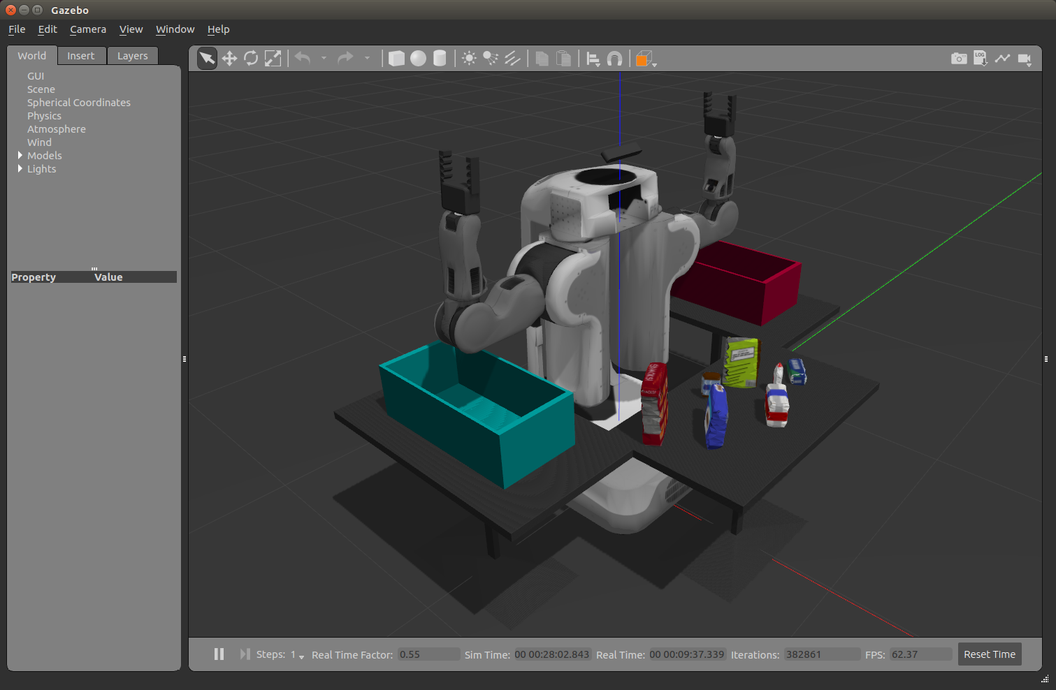
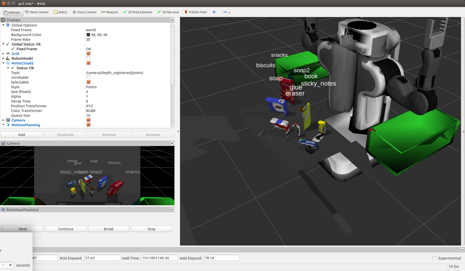
The goal of this project was to create a 3D Perception Pipeline to identify and label the table objects using the PR2 RGBD (where D is Depth) camera.

Exercise 1, 2 and 3 Pipeline Implemented

For this project the combined pipeline was implemented in perception_pipeline.py

Complete Exercise 1 steps. Pipeline for filtering and RANSAC plane fitting implemented.

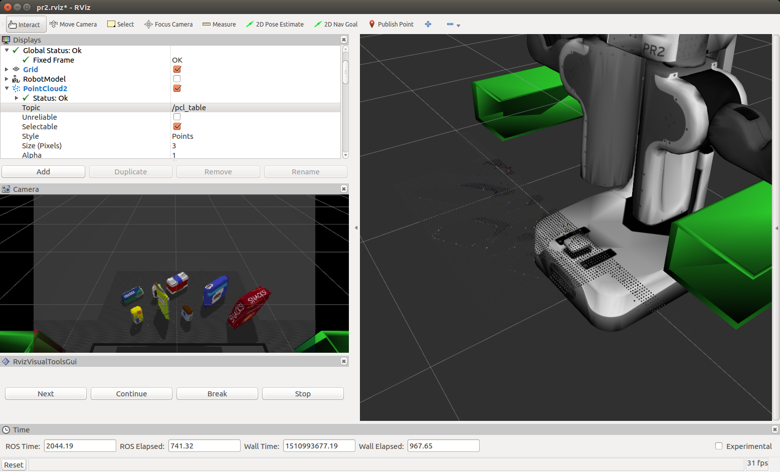
The 3D perception pipeline begins with a noisy pc2.PointCloud2 ROS message. A sample animated GIF follows:

Noisy Camera Cloud
Noisy Camera Cloud

After conversion to a PCL cloud a statistical outlier filter is applied to give a filtered cloud.

The cloud with inlier ie outliers filtered out follows:

Cloud Inlier Filtered

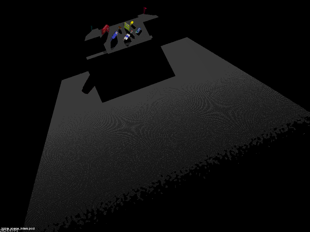
A voxel filter is applied with a voxel (also know as leaf) size = .01 to down sample the point cloud.

Voxel Downsampled
Voxel Downsampled

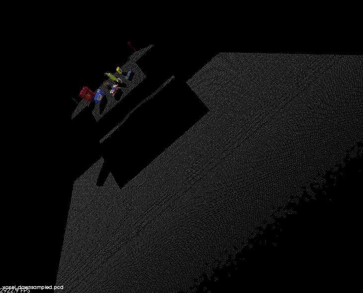
Two passthrough filters one on the ‘x’ axis (axis_min = 0.4 axis_max = 3.) to remove the box edges and another on the ‘z’ axis (axis_min = 0.6 axis_max = 1.1) along the table plane are applied.

Passthrough Filtered

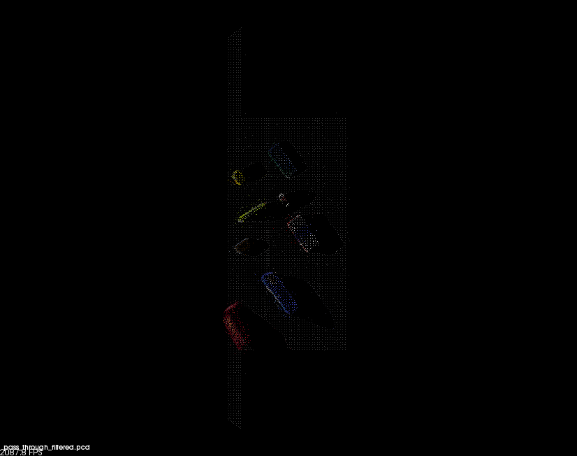
Finally a RANSAC filter is applied to find inliers being the table and outliers being the objects on it per the following

# Create the segmentation object
seg = cloud_filtered.make_segmenter()

# Set the model you wish to fit
seg.set_model_type(pcl.SACMODEL_PLANE)
seg.set_method_type(pcl.SAC_RANSAC)

# Max distance for a point to be considered fitting the model
max_distance = .01
seg.set_distance_threshold(max_distance)

# Call the segment function to obtain set of inlier indices and model coefficients
inliers, coefficients = seg.segment()

# Extract inliers and outliers
extracted_inliers = cloud_filtered.extract(inliers, negative=False)
extracted_outliers = cloud_filtered.extract(inliers, negative=True)
cloud_table = extracted_inliers
cloud_objects = extracted_outliers

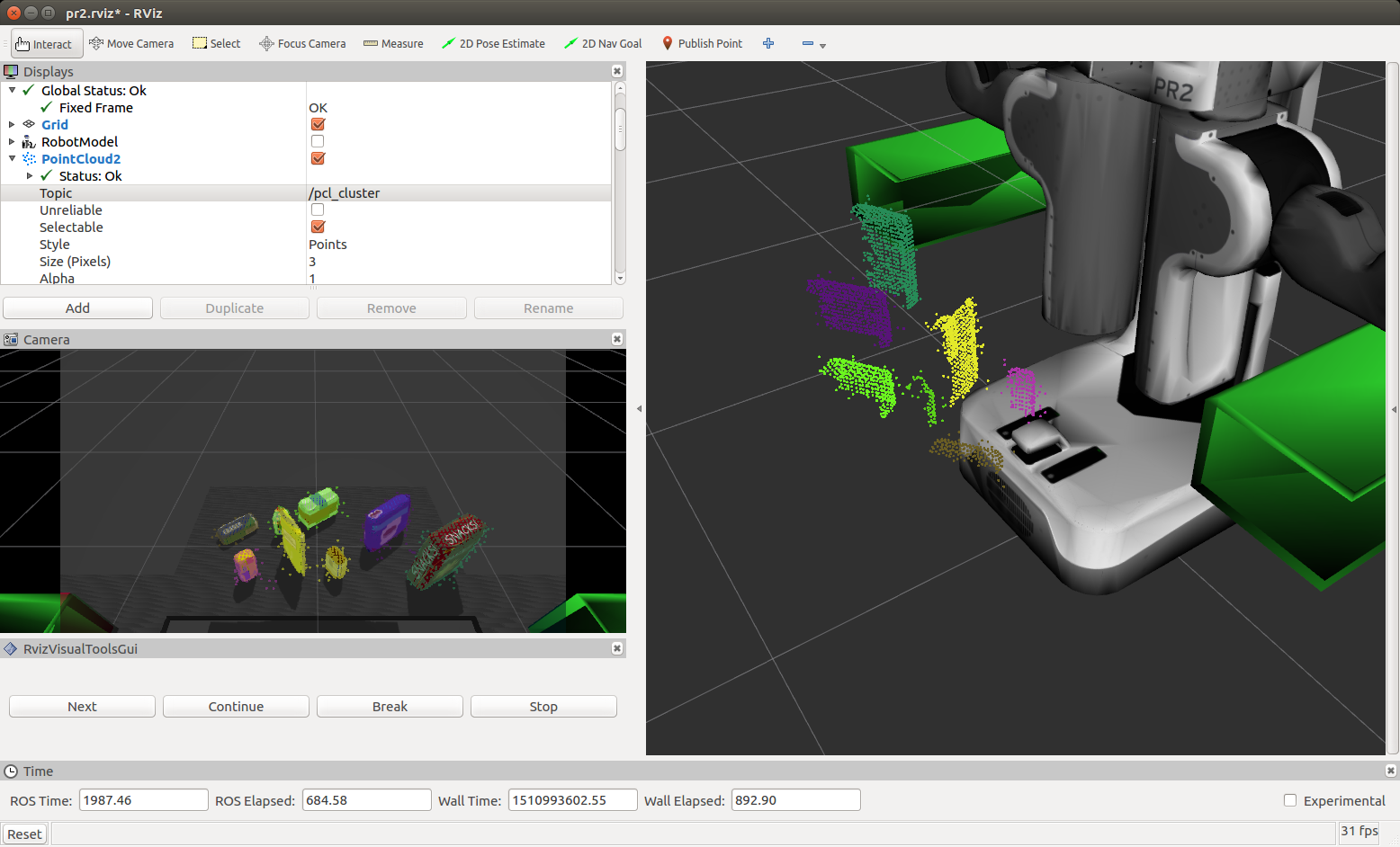
Complete Exercise 2 steps: Pipeline including clustering for segmentation implemented.

Euclidean clustering on a white cloud is used to extract cluster indices for each cluster object. Individual ROS PCL messages are published (for the cluster cloud, table and objects) per the following code snippet:

    # Euclidean Clustering
    white_cloud = XYZRGB_to_XYZ(cloud_objects)
    tree = white_cloud.make_kdtree()

    # Create a cluster extraction object
    ec = white_cloud.make_EuclideanClusterExtraction()

    # Set tolerances for distance threshold
    # as well as minimum and maximum cluster size (in points)
    ec.set_ClusterTolerance(0.03)
    ec.set_MinClusterSize(30)
    ec.set_MaxClusterSize(1200)
    # Search the k-d tree for clusters
    ec.set_SearchMethod(tree)
    # Extract indices for each of the discovered clusters
    cluster_indices = ec.Extract()

    # Create Cluster-Mask Point Cloud to visualize each cluster separately
    #Assign a color corresponding to each segmented object in scene
    cluster_color = get_color_list(len(cluster_indices))

    color_cluster_point_list = []

    for j, indices in enumerate(cluster_indices):
        for i, indice in enumerate(indices):
            color_cluster_point_list.append([white_cloud[indice][0],
                                            white_cloud[indice][1],
                                            white_cloud[indice][2],
                                            rgb_to_float(cluster_color[j])])

    #Create new cloud containing all clusters, each with unique color
    cluster_cloud = pcl.PointCloud_PointXYZRGB()
    cluster_cloud.from_list(color_cluster_point_list)

    # Convert PCL data to ROS messages
    ros_cloud_objects = pcl_to_ros(cloud_objects)
    ros_cloud_table = pcl_to_ros(cloud_table)
    ros_cluster_cloud = pcl_to_ros(cluster_cloud)

    # Publish ROS messages
    pcl_objects_pub.publish(ros_cloud_objects)
    pcl_table_pub.publish(ros_cloud_table)
    pcl_cluster_pub.publish(ros_cluster_cloud)
/pcl_objects
/pcl_objects
/pcl_table
/pcl_table
/pcl_cluster
/pcl_cluster

Complete Exercise 3 Steps. Features extracted and SVM trained. Object recognition implemented.

Features were captured in the sensor_stick simulator for [‘biscuits’, ‘soap’, ‘soap2’, ‘book’, ‘glue’, ‘sticky_notes’, ‘snacks’, ‘eraser’] model names with 40 sample of each captures.

hsv color space was used a combination of color and normalised histograms per

# Extract histogram features
chists = compute_color_histograms(sample_cloud, using_hsv=True)
normals = get_normals(sample_cloud)
nhists = compute_normal_histograms(normals)
feature = np.concatenate((chists, nhists))
labeled_features.append([feature, model_name])

The colour histograms where produced with 32 bins in the range (0, 256) and the normal values with 32 bins in the range (-1, 1.).
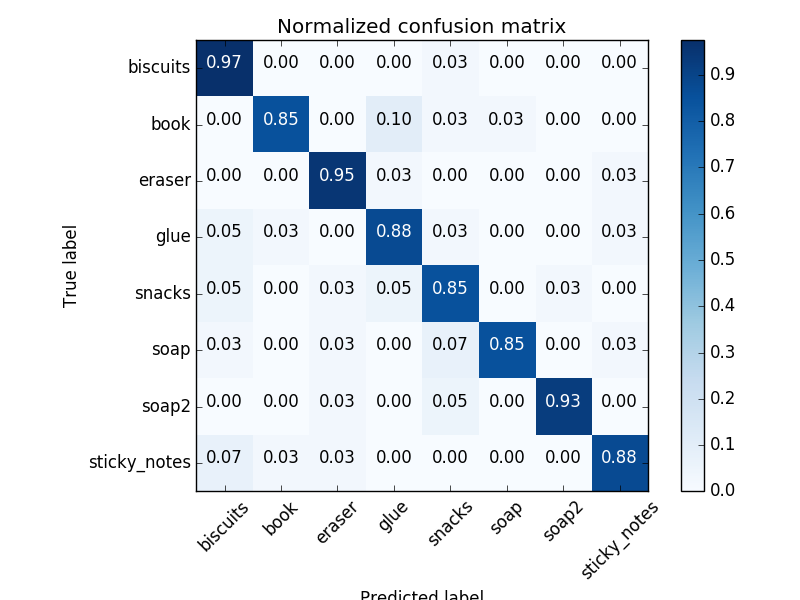
The full training.set was used in train_svm.py where I replaced the standard sum.SVC(kernel='linear') classifier with a Random Forest based classifier.

clf = ExtraTreesClassifier(n_estimators=10, max_depth=None,
                           min_samples_split=2, random_state=0)

It dramatically improved training scores per the following normalised confusion matrix:

normalised confusion matrix

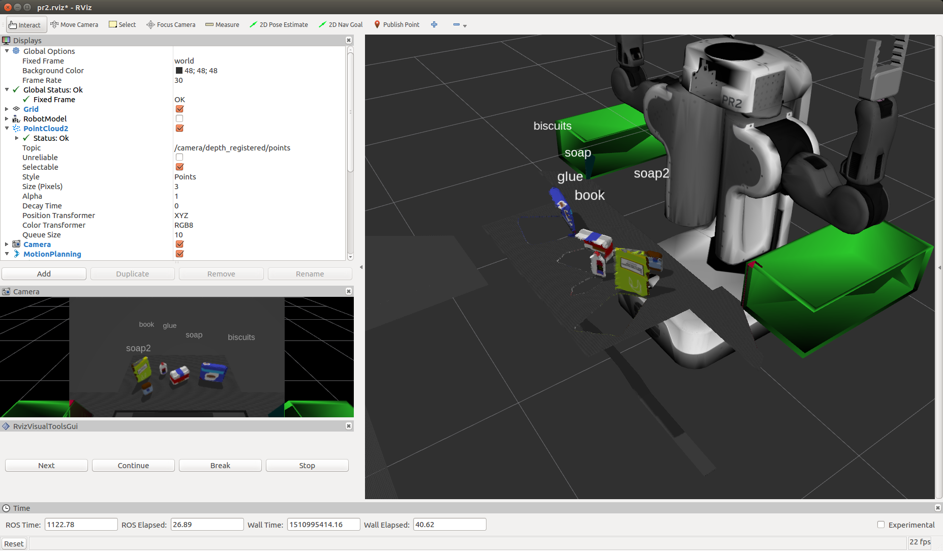
The trained model.sav was used as input into the perception pipeline where for each cluster found in the point cloud, histogram features were extracted as per the training step above and used in prediction and added to a list of detected objects.

# Make the prediction, retrieve the label for the result
# and add it to detected_objects_labels list
prediction = clf.predict(scaler.transform(feature.reshape(1, -1)))
label = encoder.inverse_transform(prediction)[0]

Pick and Place Setup

test1.world

labeled test1 output

output_1.yaml

test2.world

labeled test2 output

output_2.yaml

test3.world

labeled test3 output

output_3.yaml

Reflection

It was interesting to learn about using point clouds and to learn this approach. I found occasionally there was some false readings. In addition few of the objects were picked and placed in the crates (the PR2 did not seem to grasp them properly). This may mean that further effort is needed to refine the centroid selection of each object.

Whilst I achieved average ~90% accuracy, across all models, on the classifier training, with more time spent, I would have liked to have achieved closer to 97%. This would also improve those false readings. I’m also not sure I fully understand the noise introduced in this project from the PR2 RGBD camera.

If I was to approach this project again, I’d be interested to see how a 4D Tensor would work via deep learning using YOLO and/or CNNs. Further research is required.

Search and Sample Return

Robotics Nano Degree

Udacity - Robotics NanoDegree Program


Rover simulator output

The goal of this project were to use perception and decision steps to control a rover in a simulator. Perception occurs via using computer vision techniques to determine navigable terrain and then make decisions to take Action on the rover.

Its the first project of the Robotics Nano Degree program. I ran my simulator in 1600×1200 resolution. Different resolution may impact on the performance of the model in this project.

Notebook Analysis

The first step was to perform some analysis in a jupyter notebook on sample/calibration data.

Run the functions provided in the notebook on test images (first with the test data provided, next on data you have recorded). Add/modify functions to allow for color selection of obstacles and rock samples.

This step involved loading the data

Calibration data with grid
Rock Sample

and then doing a perspective transform to get a birds eye view.

Warped Example
Warped Rock

A function color_thresh was provided to do color thresholding (defaulted to RGB channels > 160). It was used as the basis to create an obstacle_thresh method (which selected the inverse ie RGB color channels <= 160). A rock_thresh method was created that selected between min and max color channels. The image color channels are converted from RGB to YUV before being used via warped_rock_yuv=cv2.cvtColor(warped_rock, cv2.COLOR_RGB2YUV).

Warped Threshed (white shows what is navigatable)
Obstacle Threshed (white shows obstacle)
Rock Threshed (white shows rock)

Populate the process_image() function with the appropriate analysis steps to map pixels identifying navigable terrain, obstacles and rock samples into a worldmap. Run process_image() on your test data using the moviepy functions provided to create video output of your result.

1) Define source and destination points for perspective transform
dst_size = 5 
bottom_offset = 6
source = np.float32([[14, 140], [301 ,140],[200, 96], [118, 96]])
destination = np.float32([[img.shape[1]/2 - dst_size, img.shape[0] - bottom_offset],
              [img.shape[1]/2   dst_size, img.shape[0] - bottom_offset],
              [img.shape[1]/2   dst_size, img.shape[0] - 2*dst_size - bottom_offset], 
              [img.shape[1]/2 - dst_size, img.shape[0] - 2*dst_size - bottom_offset],
              ])
2) Apply perspective transform

a warped image is created using the source and destination points from above warped = perspect_transform(img, source, destination)

3) Apply color threshold to identify navigable terrain/obstacles/rock samples

The thresh_min and thresh_max values were determined via an interactive cell in the notebook.

threshed = color_thresh(warped)
obstacle_threshed = obstacle_thresh(warped)
warped_yuv=cv2.cvtColor(warped, cv2.COLOR_RGB2YUV)
thresh_min=(0, 38, 153)
thresh_max=(145, 148, 170)
rock_threshed = rock_thresh(warped_yuv, thresh_min, thresh_max)
4) Convert thresholded image pixel values to rover-centric coords
xpix, ypix = rover_coords(threshed)
xpix_obst, ypix_obst = rover_coords(obstacle_threshed)
xpix_rock, ypix_rock = rover_coords(rock_threshed)
5) Convert rover-centric pixel values to world coords
world_size = data.worldmap.shape[0]
scale = 12
xpos = data.xpos[data.count]
ypos = data.ypos[data.count]
yaw = data.yaw[data.count]

xpix_world, ypix_world = pix_to_world(xpix, ypix, xpos, ypos, yaw, world_size, scale)
xpix_world_obst, ypix_world_obst = pix_to_world(xpix_obst, ypix_obst, xpos, ypos, yaw, world_size, scale)
xpix_world_rock, ypix_world_rock = pix_to_world(xpix_rock, ypix_rock, xpos, ypos, yaw, world_size, scale)

note: data.count contains the current position in index for the video stream.

6) Update worldmap (to be displayed on right side of screen)
for obstacle_x_world, obstacle_y_world in zip (xpix_world_obst, ypix_world_obst):
    data.worldmap[obstacle_y_world, obstacle_x_world, 0]  = 1
for rock_x_world, rock_y_world in zip (xpix_world_rock, ypix_world_rock):
    data.worldmap[rock_y_world, rock_x_world, 1]  = 1
for navigable_x_world, navigable_y_world, in zip(xpix_world, ypix_world):
    data.worldmap[navigable_y_world, navigable_x_world, 2]  = 1
7) Make a mosaic image

A mosaic image was created showing the rover camera image, warped image, ground truth (with rover location and direction arrow) and another ground truth (showing the current obstacle and navigable mapping)

Test video follows

Test Mapping Video

Test Mapping Video MP4

Autonomous Navigation and Mapping

Fill in the perception_step() (at the bottom of the perception.py script) and decision_step() (in decision.py) functions in the autonomous mapping scripts and an explanation is provided in the writeup of how and why these functions were modified as they were.

perception_step()

This step utilised the efforts from the notebook analysis, described above. The Rover Worldmap was not updated if there was observable pitch or roll (eg > or – 1 degree).

In addition rover polar coordinates were derived and saved against the passed Rover object for both navigable areas and observed rocks (if no rocks observed set to None).

decision_step()

This is the challenging part of the project.

stop and forward were the two default rover modes supplied. For this project stuck, rock and reverse were added.

forward was modified to have a left hugging biases by adding 65% of the standard deviation of the navigable angles, as long as there had been some travel time either initially or after being stuck.

The rover enters stuck mode if the rover stays in the same position, whilst not picking up a rock, for 5 seconds. If still stuck after 10 seconds, then reverse mode is tried. After 15 seconds, stuck and reverse are reset before trying stop mode.

stuck mode tries rotating if there is an obstruction in front, moving forward if steering not locked full left or right whilst going slow, and breaking if steering is locked full left or right. It will reset to forward if movement is restored.

reverse mode rotates randomly between 30 and 180 degrees after setting the brakes and reducing velocity to zero. Once its within or – 15 degrees it sets mode to forward. If reverse mode is in-affective to sets it to stop mode.

If a rock is observed, some false positives are ignored, as well as distant rocks before being placed into rock mode. Whilst the rock is not close, it tries to navigate closer towards it before breaking or coasting closer. The algorithm still requires more refinement.

Note: All my testing and running in Autonomous mode was done at 1600×1200 resolution.