Map My World Robot

Abstract

The third project in term 2 of the Udacity Robotics Nano Degree program requires students to use ROS and Gazebo along with RTAB-Map, to create a 2D occupancy grid and a 3D octomap of two environments – one supplied and the other student created.

Students extend a previous robot creation to upgrade sensors to supply the necessary sensor messages for RTAB-Map. This leverages the laser scanner, IMU/Wheel Encoder but replaces the camera with a RGB-D camera (ie kinect).

Further the ROS project is created with all links connected with appropriate naming and mapping.

The robot is launched and teleoped around the room to generate a map of the environment.

After successfully mapping the supplied environment, a student defined environment is created and mapped using the same technique.

Introduction

In this project a robot model uses a Simultaneous Localisation and Mapping (SLAM) technique called RTAB-Map (Real-Time Appearance-Based Mapping). It is a RGB-D Graph Based SLAM approach that uses incremental appearance based loop closure detection.

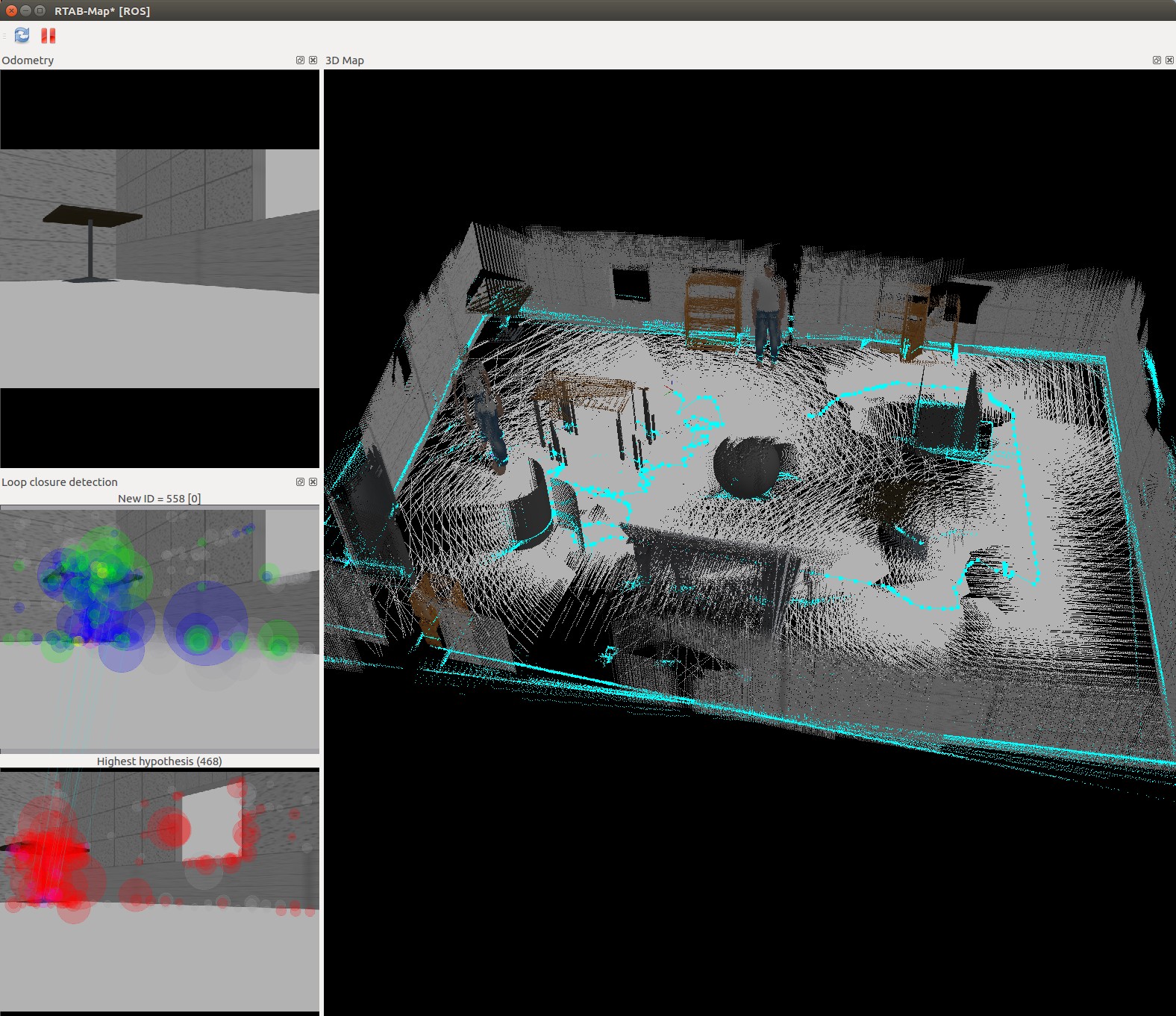
The RTAB-Map ROS wrapper is leveraged with visual representation in real time via rtabmapviz. The resultant map is stored in local database that be later interrogated via rtabmap-databaseViewer.

Background

When a robot encounters a new environment where there is no supplied map, it needs to be able to create this map and localise its pose using it. This combined localisation and mapping process is referred to as SLAM (Simultaneous Localisation and Mapping).

The main mapping algorithms are Occupancy Grid Mapping, Grid-based FastSLAM, Graph-SLAM and RTAB-Map.

The Occupancy Grid Mapping is a 2D algorithm where each grid cell is identified as Unknown/Undiscovered Zone, Free Zone or Occupied. This represents a slice of the 3D world.

The Grid-Based FastSLAM approach combines SLAM (Synchronised Location and Mapping) using a MCL (Monte Carlo Localisation) Algorithm and an Occupancy Grid Mapping. The main advantage of is the MCL particle filter approach but it always assumes there are known landmark positions. Thus it is unable to model an arbitrary environment.

Graph-SLAM uses a graph based approach to represent poses, features from the environment, motion constraints (between two poses) and measurement constraints (ties together a feature and a pose). It solves the full SLAM problem, it covers the entire path and map and not the most recent pose.

This project uses RTAB-Map, which is a Graph-SLAM approach that uses loop closure with Visual Bag-of-Words for optimisation.

The loop closure detection occurs against working memory to constrain the number of images interrogated. Working memory can be transferred and retrieved from long term memory to reduce complexity. The algorithm used for loop closure detection is SURF (Speeded Up Robust Features).

The possible outputs of RTAB-Map are 2D occupancy grid map, 3D octomap or a 3D point cloud.

Robots are of varying dimensions inclusive of height. Whilst mapping a 2d environment may show where fixed walls etc are it does not take into account height. A robot, that is propelled on the floor, may be able to navigate under some obstacles but not others eg a chair vs a large table. Hence the need to understand the environment from a 3D perspective.

However building a 3D map is more costly then a 2D map. This is not only in terms of Compute & Data costs but also in the cost of the sensors required. However, simple sensors such as a single camera may be cheaper but the algorithms required can be more complex.

Robot Model Configuration

The robot model used was based on the nick_bot created in the previous project as the student robot model (which had a square base with two actuators for the left and right wheels). The camera was removed and replaced with a kinect leveraging the openni_camera ros package with the gazebo controller Openni Kinect.

No changes were made to the hokuyo laser range finder.

An additional joint was added to rotate the kinect data 180%. It was positioned on the front of the robot so as to not interfere with the laser range finder.

The nick_bot configuration files can be found under the urdf directory.

Visualization of the frames follows

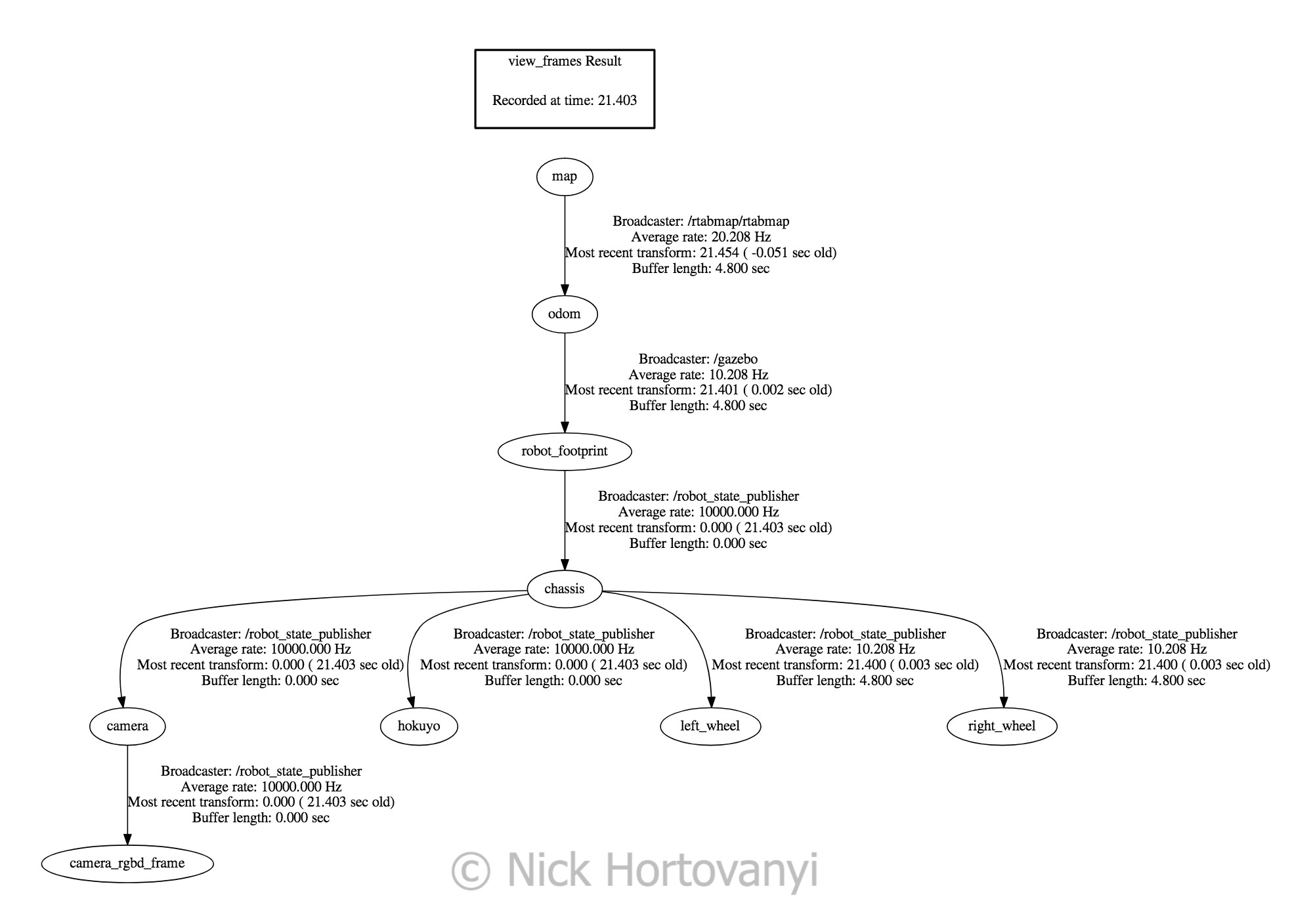
frames.png

World Creation

Two worlds were created in gazebo – one supplied as kitchen_dining.world and the other student customised nicks_building.world

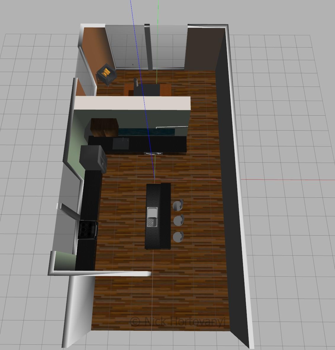
kitchen_dining.world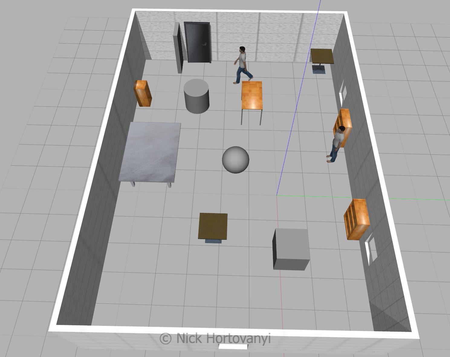

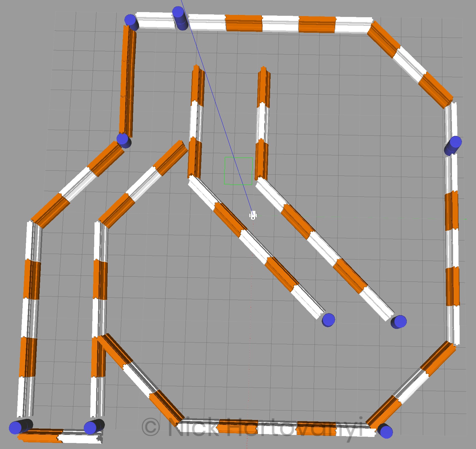
nicks_building.world

Fixtures were selected in nicks_building.world to give sufficient points for the SLUR algorithm to detect distinct points. Items were also placed to ensure that the features could not be mistakenly detected twice ie a person was placed next to one of the bookshelves. Sufficient space was left for the robot to navigate.

The following tree diagram depicts the package structure and files that made it up.

├── CMakeLists.txt
├── launch
│   ├── config
│   │   └── robot_slam.rviz
│   ├── mapping.launch
│   ├── robot_description.launch
│   ├── rviz.launch
│   ├── teleop.launch
│   └── world.launch
├── materials
│   └── textures
│       └── kinect.png
├── meshes
│   ├── hokuyo.dae
│   └── kinect.dae
├── output
│   └── rtabmap.db
├── package.xml
├── README.md
├── rtab_run
├── teleop
├── urdf
│   ├── nick_bot.gazebo
│   └── nick_bot.xacro
└── worlds
    ├── kitchen_dining.world
    └── nicks_building.world

This tree structure was chosen based on the previous student project that conformed to known gazebo/ros standards with the addition of an output directory to store Udacity project writeup requirements.

Results

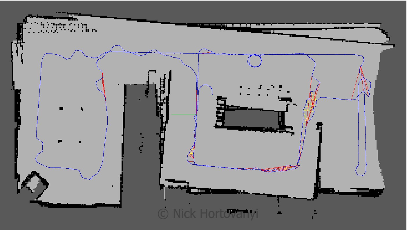
kitchen_dining_3d

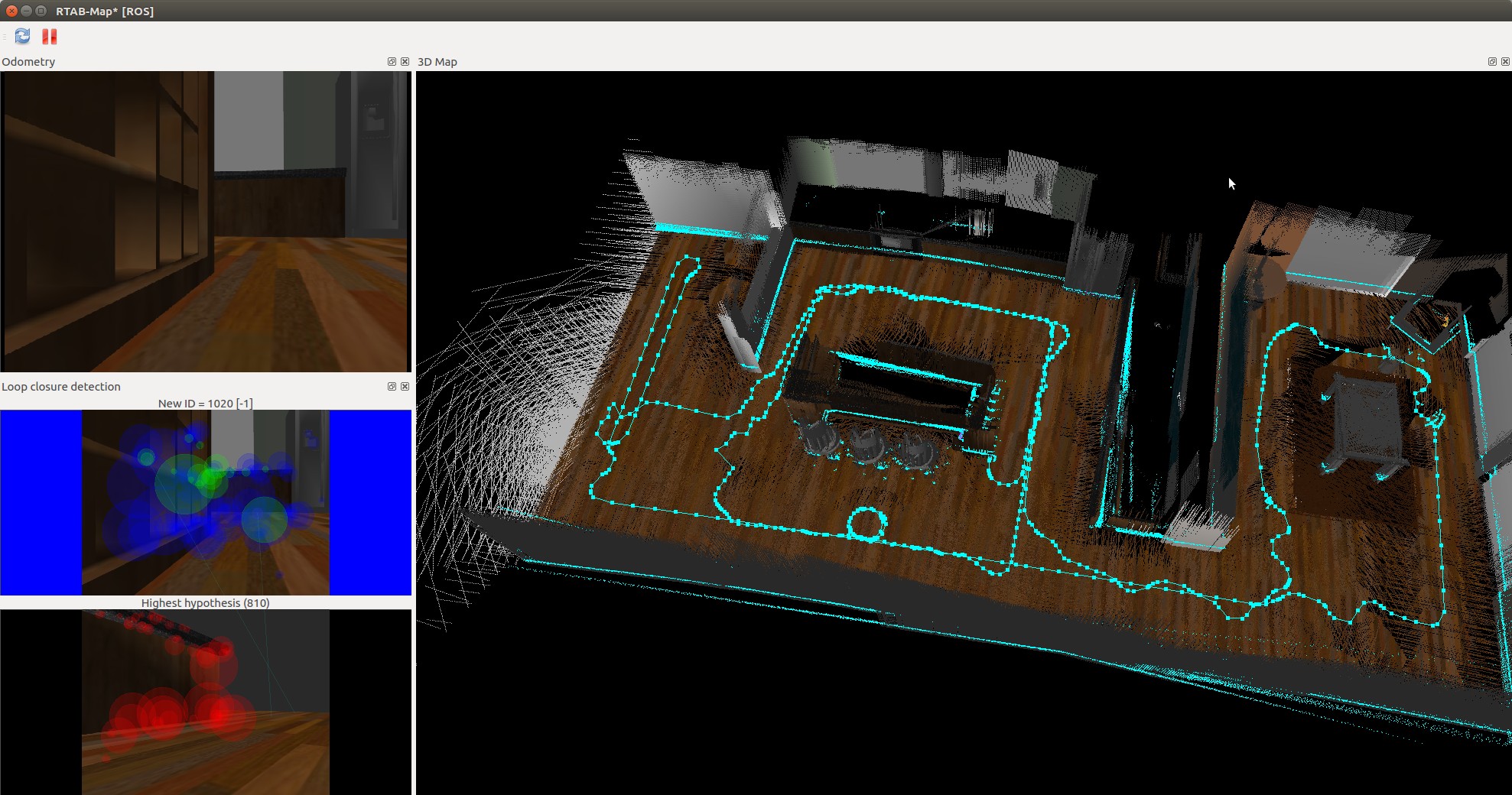
kitchen_dining_2d

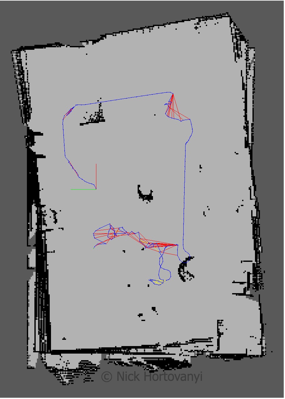
nicks_building_3d

nicks_building_2d

Discusion

The robot was teleoped (navigated via the keyboard) around the room. At some points the robot did not move forward. This appeared to be when it started to perform loop closure. Kp/MaxFeatures was halved to 200 and Vis/MinInliers was reduced from 15 to 10.

However the 3D map quickly started to resemble the physical kitchen dining gazebo model. To improve loop detection rates some, on the spot circles were performed. Of particular note were the features in the main kitchen area. More SURF features were identified there as there was more variation in the surface s.

The nick building gazebo model wall surfaces were tiled, repeatable pattern with lack of other discerning features sometimes caused the loop closure detection to map to an incorrect previous image. This then distorted the map. Additional features were added to achieve a successful map.

The kitchen_dining model performed significantly better then the student created nicks_building model. This was due to the richer and more complex features of the kitchen_dining model.

Future Work

Mapping is important to help understand the world. There are a plethora of sensors and of interest is the about to arrive solid state lidars. As the price point of these sensors continues to drop it will open up opportunities to create richer and more realistic 3D maps at a cheaper price point.

Being able to map an environment cost effectively to create a replicated virtual world will increasingly be important to allow for the training of deep learning models. We are actively looking to do this and then supplant the trained model back into a robot so it can navigate in the original environment that was mapped.

Where am I

Where am I? Project Writeup

Abstract

The second project in term 2 of the Udacity Robotics Nano Degree program requires students to complete a hijacked robot scenario using ROS and Gazebo.

Students are to initially follow instructions for a building a reference robot model, before tuning the localisation parameters satisfactorily such that the robot within the Gazebo maze simulation can reach an end goal.

After completion of that, a new robot model is created with alterations to the base and position of sensors. Whereby it uses the same simulation and must reach the same end goal.

Introduction

In this project a robot model has to use localisation to work out where it is. It creates a rolling local map using laser range sensors. The local map in turn is used to navigate towards a navigation goal.

The navigation stack utilised move_base. It provides a local cost map, as the robot moves, in relation to a global cost map to define a continuous path for the robot to move along.

This project utilises Gazebo to create a simulation with a map provided by Clearpath Robotics

Once the robot has reached the navigation goal, the objective of the project has been achieved.

Background

A robot needs to understand where it is in a world, to be able to make navigation plans to get from point a, to point b, whilst avoiding obstacles. The process of understanding “where am I?” (from a robots perspective) is called localisation.

This project uses a localisation package built into ROS called Adaptive Monte Carlo Localisation (AMCL) to assist with the robot in a scenario to work out where it is. Hence the project name “Where am I?”.

AMCL is a variant of the Monte Carlo Localisation (MCL) which was learnt in the course material. MCL uses particles to localise the robot pose. It has several advantages over using Extended Kalman Filters (EKF) such as uses raw measurements (ie from lasers), is not reliant on gaussian noise, is memory and time efficient, and can perform global localisation.

The AMCL package adaptively alters the number of particles used, which has the advantage of reducing the computational overhead required.

Results

We first completed this exercise using the class room example which is named udacity_bot. Then a different version was created where the base and sensor locations were changed. This was named nick_bot and was launched using udacity_world_nick.launch.

The final results of when it reached the goal state follow.

udacity_bot

udacity_bot rviz

nick_bot

nick_bot rviz

Model Configuration

This discussion is for the configuration of nick_bot.

The nick_bot was a square version of the rectangle based udacity_bot. The laser sensor was moved to the front of the robot.

The amcl_nick.lauch. Wherever possible the same configuration and parameters as the udacity_bot used amcl.launch.

min_particles was set to 25 and max_particles to 200 to not heavily utilise CPU. A higher max_particles did not improve initial ability of the robot to find itself with certainty.

odom_alpha1 to odom_alpha4 were trial & error values and changed from the default of 0.2 (there was not much documentation about).

The laser model parameters were left as default. There appeared no reason to change them as they were clearly visible on the above rviz visualisations and aligned to the barriers.

The yaw_goal_tolerance and xy_goal_tolerance were doubled from the default values to allow for additional flexibility in trajectory planning.

costmap_common_params_nick.yaml

transform_tolerance was set 1.25 and update_frequency to 3.0 for both local and global.

obstacle_range was set to 1.5, raytrace_range to 4.0 and inflation_radius to 0.65 to enable sufficient space on the cost map for the robot to navigate.

robot_radius was set to 0.4 in this model to allow for the larger square design.

local_costmap_params.yaml

The local publish_frequency was set to 3.0 with the global to 5.0 This configuration in conjunction with 15.0 x 15.0 sized local cost map was able to function within the performance constraints of the system used. Increasing the size of the local cost map utilise significant more computer power and missed the time windows for publish_frequency.

global_costmap_params.yaml

the update and publish frequency were set per above. In addition the width and height were set to the map size.

base_local_planner_params.yaml

sim_time was set to 4 as there appeared sufficient compute resource to estimate a trajectory out 4 seconds.

meter_scoring was enabled to ensure pdist_scale used meters.

pdist_scale was set to 0.5 being less than the default of 0.6. Default and higher values appeared to cause the robot to sometimes get stuck.

Discussion

The robot model was able to on most runs navigate successfully to the goal. The route taken at times could have been shortened. However further research is required into the ROS packages used to be able to tune it to achieve such. Often the observed path taken did not appear to be the most cost affective and when it missed the target goal, it would do a large sweep before re-approaching the target.

The AMCL routine appeared to quickly gain certainty about the locality of the robot. It was the rest of the navigation stack and move_base that needed further tuning.

In the kidnapped robot problem where by a robot is positioned in an arbitrary location, AMCL would be able to adapt the number of particles used to gain certainty of the robot’s location. In addition AMCL does not rely on landmarks, but on laser based maps, laser scans and transform messages to output pose estimates.

Moreover in an environment, where by there weren’t known landmarks, the AMCL has advantages over the Extended or Unscented Kalman Filter based approaches. These environments would include those with no known map (ie its the first time being navigated) or in highly unstructured environments with lots of moving structures over time eg shopping centres with popup shops in the aisles with significant foot traffic.

Future Work

The size of the local cost map had a significant impact on performance. Higher values decreased the ability to publish within the frequency required. In addition higher particle numbers whilst increasing CPU load did not reduce the time taken for the AMCL to be certain about the robots locality.

A square designed robot model as opposed to a rectangular design appeared to enable the robot to rotate more affectively around its base. Other wheel components are available but they did not publish ODOM information. Hence additional sensors might be required with further investigation into the impact of the removal of ODOM readings required.

A laser GPU gazebo component was available. This may enable reduced CPU load by moving the workload to the GPU.

A LIDAR unit would give a more complete map of the world around the robot. One could also look to include more laser sensors to map behind and to either side of the robot. This should facilitate with the creation of a more complete motion plan without the need for the robot to map it first.

When implementing this type of project on real hardware, the mobile nature of a robot, requiring it also to contain its own power sources, means that efficient usage of a CPU and GPU are a must. The higher the utilisation, the less effective time the robot will have to perform activities.

Thus whilst implementing more sensors may provide a more detailed and accurate map, in the field this would further drain the power source. Hence careful consideration is needed for the number of sensors, the total power consumption of the sensors and compute work loads, as well as the impact the quantity of data has to the compute utilisation rates whilst mobile.

If there no significant improvement in performance for the design objective and operational goals of the robot, then a more minimalist sensor and localisation cost map configuration may be appropriate.

Search and Sample Return

Robotics Nano Degree

---

Rover simulator output

The goal of this project were to use perception and decision steps to control a rover in a simulator. Perception occurs via using computer vision techniques to determine navigable terrain and then make decisions to take Action on the rover.

Its the first project of the Robotics Nano Degree program. I ran my simulator in 1600×1200 resolution. Different resolution may impact on the performance of the model in this project.

Notebook Analysis

The first step was to perform some analysis in a jupyter notebook on sample/calibration data.

Run the functions provided in the notebook on test images (first with the test data provided, next on data you have recorded). Add/modify functions to allow for color selection of obstacles and rock samples.

This step involved loading the data

and then doing a perspective transform to get a birds eye view.

A function color_thresh was provided to do color thresholding (defaulted to RGB channels > 160). It was used as the basis to create an obstacle_thresh method (which selected the inverse ie RGB color channels <= 160). A rock_thresh method was created that selected between min and max color channels. The image color channels are converted from RGB to YUV before being used via warped_rock_yuv=cv2.cvtColor(warped_rock, cv2.COLOR_RGB2YUV).

Warped Threshed (white shows what is navigatable)

Obstacle Threshed (white shows obstacle)

Rock Threshed (white shows rock)

Populate the process_image() function with the appropriate analysis steps to map pixels identifying navigable terrain, obstacles and rock samples into a worldmap. Run process_image() on your test data using the moviepy functions provided to create video output of your result.

1) Define source and destination points for perspective transform

dst_size = 5 
bottom_offset = 6
source = np.float32([[14, 140], [301 ,140],[200, 96], [118, 96]])
destination = np.float32([[img.shape[1]/2 - dst_size, img.shape[0] - bottom_offset],
              [img.shape[1]/2   dst_size, img.shape[0] - bottom_offset],
              [img.shape[1]/2   dst_size, img.shape[0] - 2*dst_size - bottom_offset], 
              [img.shape[1]/2 - dst_size, img.shape[0] - 2*dst_size - bottom_offset],
              ])

2) Apply perspective transform

a warped image is created using the source and destination points from above warped = perspect_transform(img, source, destination)

3) Apply color threshold to identify navigable terrain/obstacles/rock samples

The thresh_min and thresh_max values were determined via an interactive cell in the notebook.

threshed = color_thresh(warped)
obstacle_threshed = obstacle_thresh(warped)
warped_yuv=cv2.cvtColor(warped, cv2.COLOR_RGB2YUV)
thresh_min=(0, 38, 153)
thresh_max=(145, 148, 170)
rock_threshed = rock_thresh(warped_yuv, thresh_min, thresh_max)

4) Convert thresholded image pixel values to rover-centric coords

xpix, ypix = rover_coords(threshed)
xpix_obst, ypix_obst = rover_coords(obstacle_threshed)
xpix_rock, ypix_rock = rover_coords(rock_threshed)

5) Convert rover-centric pixel values to world coords

world_size = data.worldmap.shape[0]
scale = 12
xpos = data.xpos[data.count]
ypos = data.ypos[data.count]
yaw = data.yaw[data.count]

xpix_world, ypix_world = pix_to_world(xpix, ypix, xpos, ypos, yaw, world_size, scale)
xpix_world_obst, ypix_world_obst = pix_to_world(xpix_obst, ypix_obst, xpos, ypos, yaw, world_size, scale)
xpix_world_rock, ypix_world_rock = pix_to_world(xpix_rock, ypix_rock, xpos, ypos, yaw, world_size, scale)

note: data.count contains the current position in index for the video stream.

6) Update worldmap (to be displayed on right side of screen)

for obstacle_x_world, obstacle_y_world in zip (xpix_world_obst, ypix_world_obst):
    data.worldmap[obstacle_y_world, obstacle_x_world, 0]  = 1
for rock_x_world, rock_y_world in zip (xpix_world_rock, ypix_world_rock):
    data.worldmap[rock_y_world, rock_x_world, 1]  = 1
for navigable_x_world, navigable_y_world, in zip(xpix_world, ypix_world):
    data.worldmap[navigable_y_world, navigable_x_world, 2]  = 1

7) Make a mosaic image

A mosaic image was created showing the rover camera image, warped image, ground truth (with rover location and direction arrow) and another ground truth (showing the current obstacle and navigable mapping)

Test video follows

Test Mapping Video MP4

Autonomous Navigation and Mapping

Fill in the perception_step() (at the bottom of the perception.py script) and decision_step() (in decision.py) functions in the autonomous mapping scripts and an explanation is provided in the writeup of how and why these functions were modified as they were.

perception_step()

This step utilised the efforts from the notebook analysis, described above. The Rover Worldmap was not updated if there was observable pitch or roll (eg > or – 1 degree).

In addition rover polar coordinates were derived and saved against the passed Rover object for both navigable areas and observed rocks (if no rocks observed set to None).

decision_step()

This is the challenging part of the project.

stop and forward were the two default rover modes supplied. For this project stuck, rock and reverse were added.

forward was modified to have a left hugging biases by adding 65% of the standard deviation of the navigable angles, as long as there had been some travel time either initially or after being stuck.

The rover enters stuck mode if the rover stays in the same position, whilst not picking up a rock, for 5 seconds. If still stuck after 10 seconds, then reverse mode is tried. After 15 seconds, stuck and reverse are reset before trying stop mode.

stuck mode tries rotating if there is an obstruction in front, moving forward if steering not locked full left or right whilst going slow, and breaking if steering is locked full left or right. It will reset to forward if movement is restored.

reverse mode rotates randomly between 30 and 180 degrees after setting the brakes and reducing velocity to zero. Once its within or – 15 degrees it sets mode to forward. If reverse mode is in-affective to sets it to stop mode.

If a rock is observed, some false positives are ignored, as well as distant rocks before being placed into rock mode. Whilst the rock is not close, it tries to navigate closer towards it before breaking or coasting closer. The algorithm still requires more refinement.

Note: All my testing and running in Autonomous mode was done at 1600×1200 resolution.

Model Predictive Controller Project

This MPC (Model Predictive Controller) project, was the last in term 2 of the Udacity Self Driving Car Engineer Nanodegree.

---

Simulator output

This MPC (Model Predictive Controller) project, was the last in term 2 of the Udacity Self Driving Car Engineer Nanodegree.

Implementation

The Model

For this project (github repo) we used a global kinematic model, which is a simplification of a dynamic model that ignores tire forces, gravity and mass.

The state model is represented by the vehicles position, orientation angle (in radians) and velocity.

A cross track error (distance of vehicle from trajectory) and an orientation error (difference of vehicle orientation and trajectory orientation) were also included in the state model.

Two actuators were used, delta – to represent the steering angle (normalised to [-1,1]) and a – for acceleration corresponding to a throttle, with negative values for braking.

The simulator passes via a socket, ptsx & ptsy of six waypoints (5 in front, 1 near the vehicle), the vehicle x,y map position, orientation and speed (mph).

This data after being transformed into the vehicle map space, with new cross track error and orientation error calculated, is then passed into the MPC (Model Predictive Control) solve routine. It returns, the two new actuator values, with steering and acceleration (i.e. throttle) and the MPC predicted path (plotted in green in the simulator).

Constraint costs were applied to help the optimiser select an optimal update. Emphasis was placed on minimising orientation error and actuations, in particular steering (to keep the lines smooth).

   // Reference State Cost
    // TODO: Define the cost related the reference state and
    // any anything you think may be beneficial.
    // The part of the cost based on the reference state.
    for (int i = 0; i < N; i  ) {
      fg[0]  = CppAD::pow(vars[cte_start   i] - ref_cte, 2);
      fg[0]  = 2 * CppAD::pow(vars[epsi_start   i] - ref_epsi, 2);
      fg[0]  = CppAD::pow(vars[v_start   i] - ref_v, 2);
    }

    //
    // Setup Constraints
    //
    // NOTE: In this section you'll setup the model constraints.
    // Minimize the use of actuators.
    for (int i = 0; i < N - 1; i  ) {
      fg[0]  = CppAD::pow(vars[delta_start   i], 2);
      fg[0]  = CppAD::pow(vars[a_start   i], 2);
    }

    // Minimize the value gap between sequential actuations.
    for (int i = 0; i < N - 2; i  ) {
      fg[0]  = 20000 * CppAD::pow(vars[delta_start   i   1] - vars[delta_start   i], 2);
      fg[0]  = 10 * CppAD::pow(vars[a_start   i   1] - vars[a_start   i], 2);
    }

Timestep Length and Frequency

The MPC optimiser has two variables to represent the horizon into the future to predict actuator changes. They are determined by N (Number of timesteps) and dt (timestep duration) where T (time) = N * dt.

To help tune these settings, I copied the mpc_to_line project quiz, to a new project mpc_to_waypoint, and modified it to represent the initial state model to be used with the Udacity simulator. I was able to get good results looking out 3 seconds, with N = 15 and dt = 0.2. The following output are plots of 50 iterations from the initial vehicle state:

It seemed to be tracking quite nicely but speed was very slow.

However what I found, is that a horizon out 3 seconds in the simulator seemed to be too far. The faster the vehicle, the further forward the optimiser was looking. It shortly started to fail and the vehicle would end up in the lake or even worse airborne.

I tried reducing N and increasing dt. Eventually, via trial and error, I found good results where N was 8 to 10 and dt between ~0.08 to ~0.105. I eventually settled on calculating dt based on Time/N (with time set at ~.65 seconds and N on 8). If I saw the plotted MPC line coming close to the 2nd furthest plotted waypoint at higher speeds, it started to correspond, with the MPC optimiser failing.

The reference speed also played a part. To drive safely around the track, to ensure the project meets requirement, I kept it at 60 MPH.

Polynomial Fitting and MPC Preprocessing

An example plot of the track with the first way points, vehicle position and orientation follows:

To make updating easier and to provide data to be able to draw, the waypoints and the predicted path from the MPC solver, coordinates were transformed into vehicle space. This meant also that the initial position of the vehicle state, for the solver was (0 velocity in KPH * 100 ms of latency,0), which included a projection of distance travelled to cover latency, with a corresponding angle orientation of zero. These coordinates were used in the poly fit. It had an added benefit of simplifying, the derivative calculation required for the orientation error.

The following plot is the same waypoints transformed to the vehicle space map, with the arrow representing the orientation of the vehicle:

Model Predictive Control with Latency

Before sending the result back to the simulator a 100ms latency delay was implemented.

this_thread::sleep_for(chrono::milliseconds(100));

This replicated the actuation delay that would be experienced in a real-world vehicle.

I experimented with trying to understand if the ratio of dt (time interval) to latency in seconds, being near 1 (i.e. the time interval was close to the latency value), had an impact on the ability of the MPC algorithm to handle latency. Anecdotal evidence supported that; but in reality ratio values of < 1 (for this project, I had (.65/8)/.100 = .0.8125) were the reality to ensure the optimiser was able to find a solution.

As described in the previous section, the vehicle position was projected forward, the distance it would travel, to cover 100ms of latency.

However before I implemented the forward projection for latency, you could see in places where the vehicle lagged a little in its turning. The MPC, however predicted the path correctly back onto the centre line of the track per following image:

After I implemented the latency projection calculation, the vehicle was able to stay closer to center, more readily per this image:

Over all the drive around this simulator track, was smoother and lacked steering wobbles, when compared to using a PID controller.

Advanced Lane Detection

In this Advanced Lane Detection project, we apply computer vision techniques to augment video output with a detected road lane, road radius curvature and road centre offset. The video was supplied by Udacity and captured using the middle camera.

sample lane detection result

The goals / steps of this project are the following:

• Compute the camera calibration matrix and distortion coefficients given a set of chessboard images.
• Apply a distortion correction to raw images.
• Use color transforms, gradients, etc., to create a thresholded binary image.
• Apply a perspective transform to rectify binary image (“birds-eye view”).
• Detect lane pixels and fit to find the lane boundary.
• Determine the curvature of the lane and vehicle position with respect to center.
• Warp the detected lane boundaries back onto the original image.
• Output visual display of the lane boundaries and numerical estimation of lane curvature and vehicle position.

A jupyter/iPython data science notebook was used and can be found on github Full Project Repo – Advanced Lane Finding Project Notebook (Note the interactive ipywidgets are not functional on github). The project is written in python and utilises numpy and OpenCV.

Camera Calibration

Every camera has some distortion factor in its lens. The known approach to correct for that in (x,y,z) space is apply coefficients to undistort the image. To calculate this a camera calibration process is required.

It involves reading a set of warped chessboard images, converting them into grey scale images before using cv2.findChessboardCorners() to identify the corners as imgpoints.

If corners are detected then they are collected as image points imgpoints along with a set of object points objpoints; with an assumption made that the chessboard is fixed on the (x,y) plane at z=0 (object points will hence be the same for each calibration image).

In the function camera_calibrate I pass the collected objpoints, imgpoints and a test image for the camera image dimensions. It in turn uses cv2.calibrateCamera() to calculate the distortion coefficients before the test image is undistorted with cv2.undistort() giving the following result.

Pipeline (Test images)

After camera calibration a set of functions have been created to work on test images before later being used in a video pipeline.

Distortion corrected image

The undistort_image takes an image and defaults the mtx and dist variables from the previous camera calibration before returning the undistorted image.

Threshold binary images

A threshold binary image, as the name infers, contains a representation of the original image but in binary 0,1 as opposed to a BGR (Blue, Green, Red) colour spectrum. The threshold part means that say the Red colour channel( with a range of 0-255) was between a threshold value range of 170-255, that it would be set to 1.

A sample output follows.

Initial experimentation occurred in a separate notebook before being refactored back into the project notebook in the combined_threshold function. It has a number of default thresholds for sobel gradient x&y, sobel magnitude, sober direction, Saturation (from HLS), Red (from RGB) and Y (luminance from YUV) plus a threshold type parameter (daytime-normal, daytime-bright, daytime-shadow, daytime-filter-pavement).

Whilst the daytime-normal threshold worked great for the majority of images there were situations where it didn’t e.g. pavement colour changes in bright light and shadow.

Daytime Normal with noise bright light & pavement change

Daytime Normal with shadow

Other samples Daytime Bright, Daytime Shadow and Daytime Filter Pavement.

Perspective transform – birds eye view

To be able to detect the road lines, the undistorted image is warped. The function calc_warp_points takes an image’s height & width and then calculates the src and dst array of points. perspective_transforms takes them and returns two matrixes M and Minv for perspective_warp and perpective_unwarp functions respectively. The following image, shows an undistorted image, with the src points drawn with the corresponding warped image (the goal here was straight lines)

Lane-line pixel identification and polynomial fit

Once we have a birds eye view with a combined threshold we are in a position to identify lines and a polynomial to draw a line (or to search for points in a binary image).

topdown warped binary image

A histogram is created via lane_histogram from the bottom third of the topdown warped binary image. Within lane_peaks, scipy.signal is used to identify left and right peaks. If just one peak then the max bin either side of centre is returned.

calc_lane_windows uses these peaks along with a binary image to initialise a left and right instance of a WindowBox class. find_lane_window then controls the WindowBox search up the image to return an array of WindowBoxes that should contain the lane line. calc_fit_from_boxes returns a polynomial or None if nothing found.

poly_fitx function takes a fity where
fity = np.linspace(0, height-1, height) and a polynomial to calculate an array of x values.

The search result is plotted on the bottom left of the below image with each box in green. To test line searching by polynomial, I then use the left & right WindowBox search polynomials as input to calc_lr_fit_from_polys. The bottom right graphic has the new polynomial line draw with a blue search window (relates to polynomial used for the search from WindBoxes) that was used overlapping with a green window for the new.

Warped box seek and new polynomial fit

Radius of curvature calculation and vehicle from centre offset

In road design, curvature is important and its normally measured by its radius length. For a straight line road, that value can be quite high.

In this project our images are in pixel space and need to be converted into meters. The images are of US roads and I measured from this image the distance between lines (413 pix) and the height of dashes (275 px). Lane width in the US is ~ 3.7 meters and dashed lines 3 metres. Thus xm_per_pix = 3.7/413 and ym_per_pix = 3./275 were used in calc_curvature. The function converted the polynomial from pixel space into a polynomial in meters.

To calculate the offset from centre, I first determined where on the x plane, both the left lx and right rx lines crossed the image near the driver. I then calculated the xcentre of the image as the width/2. The offset was calculated such (rx - xcenter) - (xcenter - lx) before being multiple by xm_per_pix.

Final pipeline

I decided to take a more python class based approach once I progressed through this project. Inside the classes, I called the functions mentioned previously. The classes created were:

• Lane contains image processing, final calculations for view drawing and reference to left and right RoadLines. It also handled searching for initial lines, recalculations and reprocessing a line that was not sane;
• RoadLine contains a history of Lines and associated curvature and plotting calculations using weighted means; and
• Line contains detailed about the line and helper functions

Processing is triggered by setting the Lane.image variable. Convenient property methods Lane.warped, Lane.warped_decorated, lane.result and lane.result_decorated return processed images. It made it very easy to debug output using interactive ipywidgets (which don’t work on github)

Sample result images

lane.result_decorated

Lane.warped_decorated

Pipeline (Video)

Using moviepy to process the project video was simple. I also decorated the result with a frame count. The Project Video Lane mp4 on GitHub, contains the result (YouTube Copy)

Discussion

Problems/Issues faced

To some degree, I got distracted with trying to solve the issues I found in my algorithm with the challenge videos. This highlighted, that I need to improve my understanding of colour spaces, sobel and threshold combinations.

I included a basic algorithm to remove pavement colours from the images using a centre, left and right focal point. I noticed that the dust colour on the vehicle seemed to be also in the road side foliage. This however wasn’t sufficient to remove all pavement colour and didn’t work when there was a road type transition. It was very CPU intensive.

In the end, I used a combination of different methods, that used a basic noise filter on warped binary images to determine, if it was sufficient to look for a line or not. If it wasn’t it tried the next one, with the final being a vertical rectangle window crawl down the image. Where the best filter was determined for each box. Again this was CPU intensive, but worked.

Another issue faced was using the previous curvature radius to determine if this line was sane or not. The values were too jittery and when driving on a straight line, high. I decided not to pursue this.

Opportunities for improvement in the algorithm/pipeline

There is room here for some refactoring into a more Object oriented approach. This was not evident at the start of the project as to how it should be structured. I experimented a little with using Pool from multiprocessing to parallelise left and right lane searches. It didn’t make it into my final classes as for normal line searching using a polynomial, as I did not ascertain if the multiprocessing overhead, outweighed the parallelism value. Certainly potential here to use a more functional approach to give the best runtime options for parallelisation.

Other areas, include automatically detecting the src points for warp, handling bounce in the road and understanding surface height (above road) of the camera and its impact.

I thought also as I’ve kept history, I could extend the warp to include a bird’e eye representation of the car on the road and directly behind it. I did mean averaging on results for smoothing drawn lines, but this was not included in the new line calculations from the next image frames.

The algorithm could also be made to make predictions about the line when there is gaps. This would be easier with continuous lines then dashed.

Hypothetical pipeline failure cases

Pavement fixes and/or combined with other surfaces that create vertical lines near existing road lines.

It would also fail if there was a road crossing or a need to cross lanes or to exit the freeway.

Rain and snow would also have an impact and I’m not sure about night time.

Tail gating a car or a car on a tighter curve would potentially interrupt the visible camera and hence line detection.

Clone Driving Behaviour

Clone driving behaviour using Deep Learning

With this behaviour cloning project, we give steering & throttle instruction to a vehicle in a simulator based on receiving a centre camera image and telemetry data. The steering angle data is a prediction for a neural network model trained against data saved from track runs I performed.

The training of the neural net model, is achieved with driving behaviour data captured, in training mode, within the simulator itself. Additional preprocessing occurs as part of batch generation of data for the neural net training.

Model Architecture

I decided to as closely as possible use the Nvidia’s End to End Learning for Self-Driving Cars model. I diverged by passing cropped camera images as RGB, and not YUV, with adjusting brightness and by using the steering angle as is. I experimented with using 1/r (inverse turning radius) as input but found the values were too small (I also did not know the steering ratio and wheel base of the vehicle in the simulator).

Additional experimentation occurred with using comma.ai, Steering angle prediction model but the number of parameters was higher then the nvidia model and it worked off of full sized camera images. As training time was significantly higher, and initial iterations created an interesting off road driving experience in the simulator, I discontinued these endeavours.

The model represented here is my implementation of the nvidia model mentioned previously. It is coded in python using keras (with tensor flow) in model.py and returned from the build_nvidia_model method. The complete project is on github here Udacity Behaviour Cloning Project

Input

The input is 66x200xC with C = 3 RGB color channels.

Architecture

Layer 0: Normalisation to range -1, 1 (1./127.5 -1)

Layer 1: Convolution with strides=(2,2), valid padding, kernel 5×5 and output shape 31x98x24, with elu activation and dropout

Layer 2: Convolution with strides=(2,2), valid padding, kernel 5×5 and output shape 14x47x36, with elu activation and dropout

Layer 3: Convolution with strides=(2,2), valid padding, kernel 5×5 and output shape 5x22x48, with elu activation and dropout

Layer 4: Convolution with strides=(1,1), valid padding, kernel 3×3 and output shape 3x20x64, with elu activation and dropout

Layer 5: Convolution with strides=(1,1), valid padding, kernel 3×3 and output shape 1x18x64, with elu activation and dropout

flatten 1152 output

Layer 6: Fully Connected with 100 outputs and dropout

Layer 7: Fully Connected with 50 outputs and dropout

Layer 8: Fully Connected with 10 outputs and dropout

dropout was set aggressively on each layer at .25 to avoid overtraining

Output

Layer Fully Connected with 1 output value for the steering angle.

Visualisation

Keras output plot (not the nicest visuals)

Data preprocessing and Augmentation

The simulator captures data into a csv log file which references left, centre and right captured images within a sub directory. Telemetry data for steering, throttle, brake and speed is also contained in the log. Only steering was used in this project.

My initial investigation and analysis was performed in a Jupyter Notebook here.

Before being fed into the model, the images are cropped to 66×200 starting at height 60 with width centered – A sample video of a run cropped.

Cropped left, centre and right camera image

As seen in the following histogram a significant proportion of the data is for driving straight and its lopsided to left turns (being a negative steering angle is left) when using data generated following my conservative driving laps.

The log file was preprocessed to remove contiguous rows with a history of >5 records, with a 0.0 steering angle. This was the only preprocessing done outside of the batch generators used in training (random rows are augmented/jittered for each batch at model training time).

A left, centre or right camera was selected randomly for each row, with .25 angle ( for left and – for right) applied to the steering.

Jittering was applied per Vivek Yadav’s post to augment data. Images were randomly transformed in the x range by 100 pixels and in the y range by 10 pixels with 0.4 per xpixel adjusted against the steering angle. Brightness via a HSV (V channel) transform (.25 a random number in range 0 to 1) was also performed.

During batch generation, to compensate for the left turning, 50% of images were flipped (including reversing steering angle) if the absolute steering angle was > .1.

Finally images are cropped per above before being batched.

Model Training

Data was captured from the simulator. I drove conservatively around the track three times paying particular attention to the sharp right turn. I found connecting a PS3 controller allowed finer control then using the keyboard. At least once I waited till the last moment before taking the turn. This seems to have stopped the car ending up in the lake. Its also helped to overcome a symptom of the bias in the training data towards left turns. To further offset this risk, I validated the training using a test set I’d captured from the second track, which is a lot more windy.

Training sample captured of left, centre and right cameras cropped

Center camera has the steering angle and 1/r values displayed.

Validation sample captured of left, centre and right cameras cropped

Center camera has the steering angle and 1/r values displayed.

The Adam Optimizer was used with a mean squared error loss. A number of hyper-parameters were passed on the command line. The command I used looks such for a batch size of 500, 10 epochs (dropped out early if loss wasn’t improving), dropout at .25 with a training size of 50000 randomly augmented features with adjusted labels and 2000 random features & labels used for validation

python model.py --batch_size=500 --training_log_path=./data --validation_log_path=./datat2 --epochs 10 \
--training_size 50000 --validation_size 2000 --dropout .25

Model Testing

To meet requirements, and hence pass the assignment, the vehicle has to drive around the first track staying on the road and not going up on the curb.

The model trained (which is saved), is used again in testing. The simulator feeds you the centre camera image, along with steering and throttle telemetry. In response you have to return the new steering angle and throttle values. I hard coded the throttle to .35. The image was cropped, the same as for training, then fed into the model for prediction giving the steering angle.

steering_angle = float(model.predict(transformed_image_array, batch_size=1))
throttle = 0.35

Successful run track 1

Successful run track 2

note: the trained model I used for the track 1 run, is different to the one used to run the simulator in track 2. I found that the data I originally used to train a model to run both tracks, would occasionally meander on track 1 quite wildly. Thus used training data to make it more conservative to meet requirements for the projects.