This Deep Reinforcement Learning Arm Manipulation project has two objectives to achieve using a template project. Whereby to achieve each objective we create a DQN agent and define reward functions to teach a robotic arm.
The template project is based on the Nvidia open source project “jetson-reinforcement” developed by Dustin Franklin.
Robot Arm in Gazebo simulator
The two primary project objectives are:
Have any part of the robot arm touch the object of interest, with at least a 90% accuracy for a minimum of 100 runs.
Have only the gripper base of the robot arm touch the object, with at least a 80% accuracy for a minimum of 100 runs.
Written by Nick Hortovanyi
Reward functions
The reward functions are defined in ArmPlugin.cpp. The arm joints were updated using position control (as that was the programs default setting). For each joint there are two actions (either increase or decrease joint position).
REWARD_WIN was set to 0.125 (0.1 2nd objective) with REWARD_LOSS to -0.125 (-0.1 2nd objective).
If the robot gripper hit the ground a REWARD_LOSS * 10 was given and the episode ended.
Interim rewards, within the episode, were issued if there was no ground contact or 100 frames had beed exceeded.
The main interim reward was based on the distance goal delta between the gripper and the cycling prop. If a positive weighted average was derived then a REWARD_WIN was recorded otherwise REWARD_LOSS * distance to goal was issued. Thus the REWARD_LOSS was higher the further away from the goal the arm was.
For the gripper base (2nd) objective an additional REWARD_LOSS was added if the absolute average goal delta was < 0.001 to penalise no movement.
If the robot arm hit the prop, a REWARD_WIN * 10 was used for the first objective otherwise a REWARD_LOSS * 5 for the second objective if the collision was not with the gripper_middle.
However for the second objective a REWARD_WIN * 20 was issued if the collision point was gripper_middle.
Any collision ends the episode.
Hyper Parameters
Image dimensions were set to the same size as the input. Training was performed on a GTX1070 and there was no need to restrict memory usage. INPUT_WIDTH 64 INPUT_HEIGHT 64
OPTIMIZER "Adam" was chosen as it in general performs better then RMSProp whilst maintaining its advantages.
For objective 1 the LEARNING_RATE was 0.1 with REPLAY_MEMORY at 1000. The value was chosen via trial and error.
For objective 2 the LEARNING_RATE was decreased to 0.01 due to the higher REPLAY_MEMORY set at 20000. The higher REPLAY_MEMORY was used so as to allow for more discrete learning, due to the smaller surface area required to achieve a collision to meet objectives.
For both BATCH_SIZE was set to 512 (again sufficient memory on the GTX 1070).
LSTM was used USE_LSTMtrue with LSTM_SIZE256 which was set via trial and error.
Results
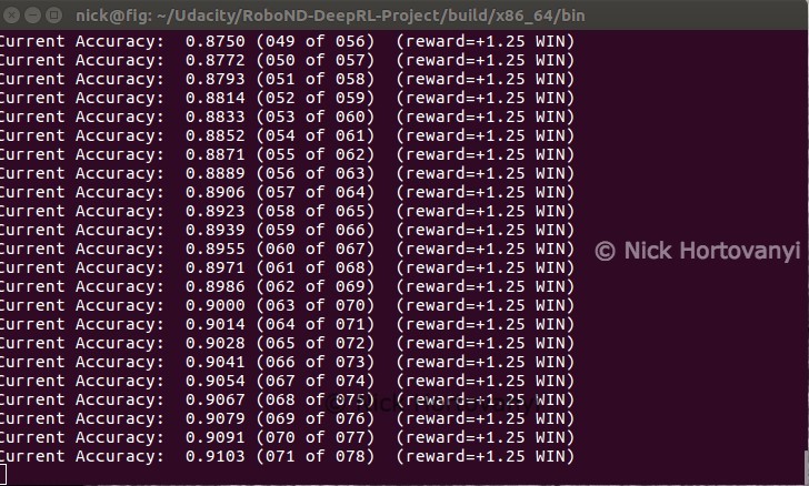
Objective 1 – Have any part of the robot arm touch the object of interest, with at least a 90% accuracy for a minimum of 100 runs.
Results objective 1
The robotic arm quickly learnt how to hit the prop with a degree accuracy in a repeatable fashion. On occasion if the arm trained initially away from the prop, it would take longer to achieve a higher accuracy.
Once a winning path was learnt this configuration consistently had the robotic arm quickly hitting the prop objective.
As can be seen in the above summary output the objective was achieved well within the criteria specified.
Objective 2 – Have only the gripper base of the robot arm touch the object, with at least a 80% accuracy for a minimum of 100 runs.
Results objective 2
With the finer control required, and alteration to the interim reward system, this configuration would often hesitate before making a move. Whilst it learnt quickly how to get very close to having the gripper_middle hit the prop, it would also often just miss either hitting the ground or the arm itself hitting the prop. There seemed to be a repeatable pattern, of just extending past and swinging down in an arch, that once learnt gave consistent winning results.
Occasionally the middle joint would collide with the ground and this would lead to the objective not being met.
This configuration was not always reproducible, however with the above screen shot it was able to meet the objectives.
Future work
There were clear arcs that once found achieved a win quickly. Such that it would be worthwhile investigating an interim reward system based on not just the distance from the goal but also distance from an ideal arc trajectory as the arm approached.
Further using centre points to calculate distance from goals becomes less accurate the closer to the goal the arm is. Such that other points like the end of the gripper_middle and top of prop cylinder, would be worthwhile experimenting with.
The third project in term 2 of the Udacity Robotics Nano Degree program requires students to use ROS and Gazebo along with RTAB-Map, to create a 2D occupancy grid and a 3D octomap of two environments – one supplied and the other student created.
Students extend a previous robot creation to upgrade sensors to supply the necessary sensor messages for RTAB-Map. This leverages the laser scanner, IMU/Wheel Encoder but replaces the camera with a RGB-D camera (ie kinect).
Further the ROS project is created with all links connected with appropriate naming and mapping.
The robot is launched and teleoped around the room to generate a map of the environment.
After successfully mapping the supplied environment, a student defined environment is created and mapped using the same technique.
Introduction
In this project a robot model uses a Simultaneous Localisation and Mapping (SLAM) technique called RTAB-Map (Real-Time Appearance-Based Mapping). It is a RGB-D Graph Based SLAM approach that uses incremental appearance based loop closure detection.
The RTAB-Map ROS wrapper is leveraged with visual representation in real time via rtabmapviz. The resultant map is stored in local database that be later interrogated via rtabmap-databaseViewer.
Background
When a robot encounters a new environment where there is no supplied map, it needs to be able to create this map and localise its pose using it. This combined localisation and mapping process is referred to as SLAM (Simultaneous Localisation and Mapping).
The Occupancy Grid Mapping is a 2D algorithm where each grid cell is identified as Unknown/Undiscovered Zone, Free Zone or Occupied. This represents a slice of the 3D world.
The Grid-Based FastSLAM approach combines SLAM (Synchronised Location and Mapping) using a MCL (Monte Carlo Localisation) Algorithm and an Occupancy Grid Mapping. The main advantage of is the MCL particle filter approach but it always assumes there are known landmark positions. Thus it is unable to model an arbitrary environment.
Graph-SLAM uses a graph based approach to represent poses, features from the environment, motion constraints (between two poses) and measurement constraints (ties together a feature and a pose). It solves the full SLAM problem, it covers the entire path and map and not the most recent pose.
This project uses RTAB-Map, which is a Graph-SLAM approach that uses loop closure with Visual Bag-of-Words for optimisation.
The loop closure detection occurs against working memory to constrain the number of images interrogated. Working memory can be transferred and retrieved from long term memory to reduce complexity. The algorithm used for loop closure detection is SURF (Speeded Up Robust Features).
The possible outputs of RTAB-Map are 2D occupancy grid map, 3D octomap or a 3D point cloud.
Robots are of varying dimensions inclusive of height. Whilst mapping a 2d environment may show where fixed walls etc are it does not take into account height. A robot, that is propelled on the floor, may be able to navigate under some obstacles but not others eg a chair vs a large table. Hence the need to understand the environment from a 3D perspective.
However building a 3D map is more costly then a 2D map. This is not only in terms of Compute & Data costs but also in the cost of the sensors required. However, simple sensors such as a single camera may be cheaper but the algorithms required can be more complex.
Robot Model Configuration
The robot model used was based on the nick_bot created in the previous project as the student robot model (which had a square base with two actuators for the left and right wheels). The camera was removed and replaced with a kinect leveraging the openni_camera ros package with the gazebo controller Openni Kinect.
No changes were made to the hokuyo laser range finder.
An additional joint was added to rotate the kinect data 180%. It was positioned on the front of the robot so as to not interfere with the laser range finder.
The nick_bot configuration files can be found under the urdf directory.
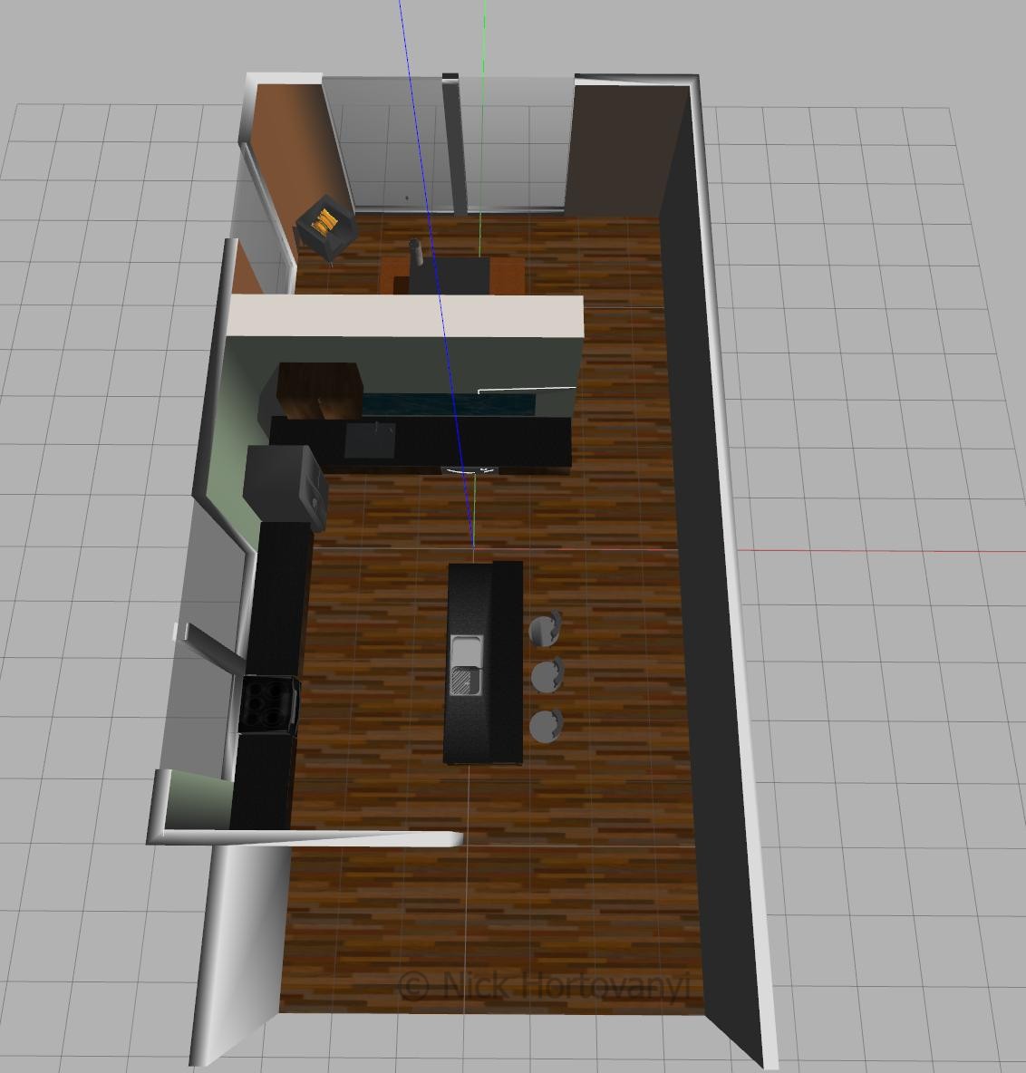
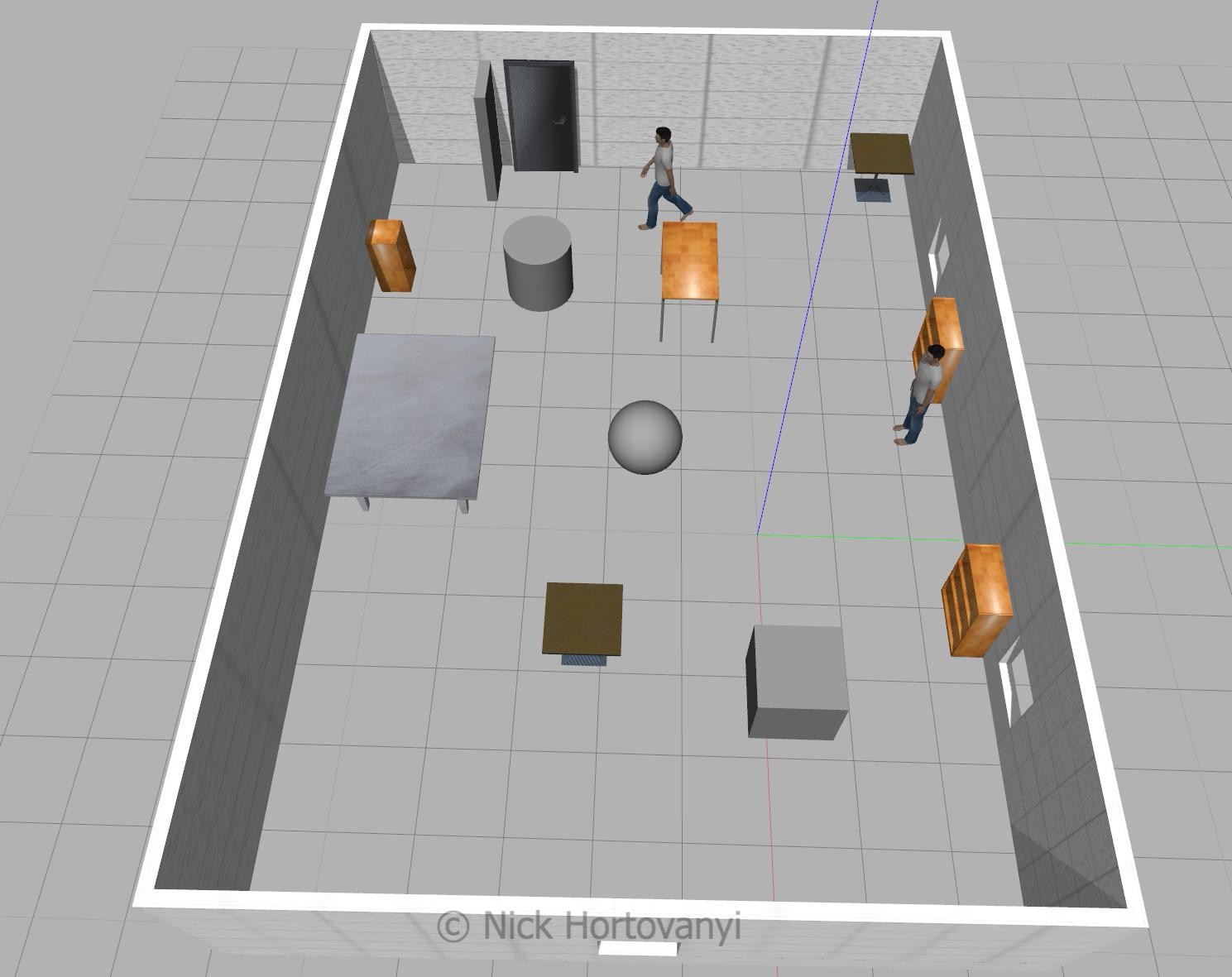
Two worlds were created in gazebo – one supplied as kitchen_dining.world and the other student customised nicks_building.world
kitchen_dining.worldnicks_building.world
Fixtures were selected in nicks_building.world to give sufficient points for the SLUR algorithm to detect distinct points. Items were also placed to ensure that the features could not be mistakenly detected twice ie a person was placed next to one of the bookshelves. Sufficient space was left for the robot to navigate.
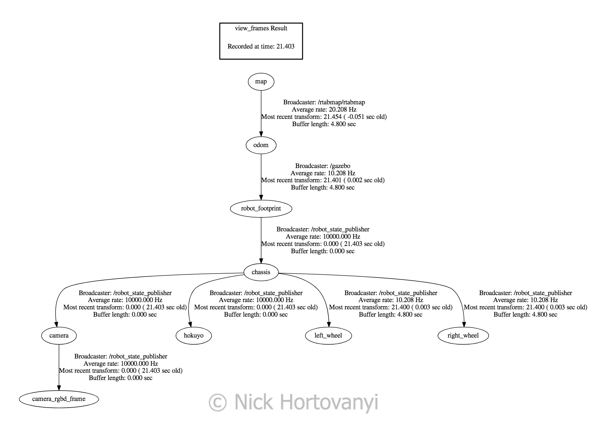
The following tree diagram depicts the package structure and files that made it up.
This tree structure was chosen based on the previous student project that conformed to known gazebo/ros standards with the addition of an output directory to store Udacity project writeup requirements.
Results
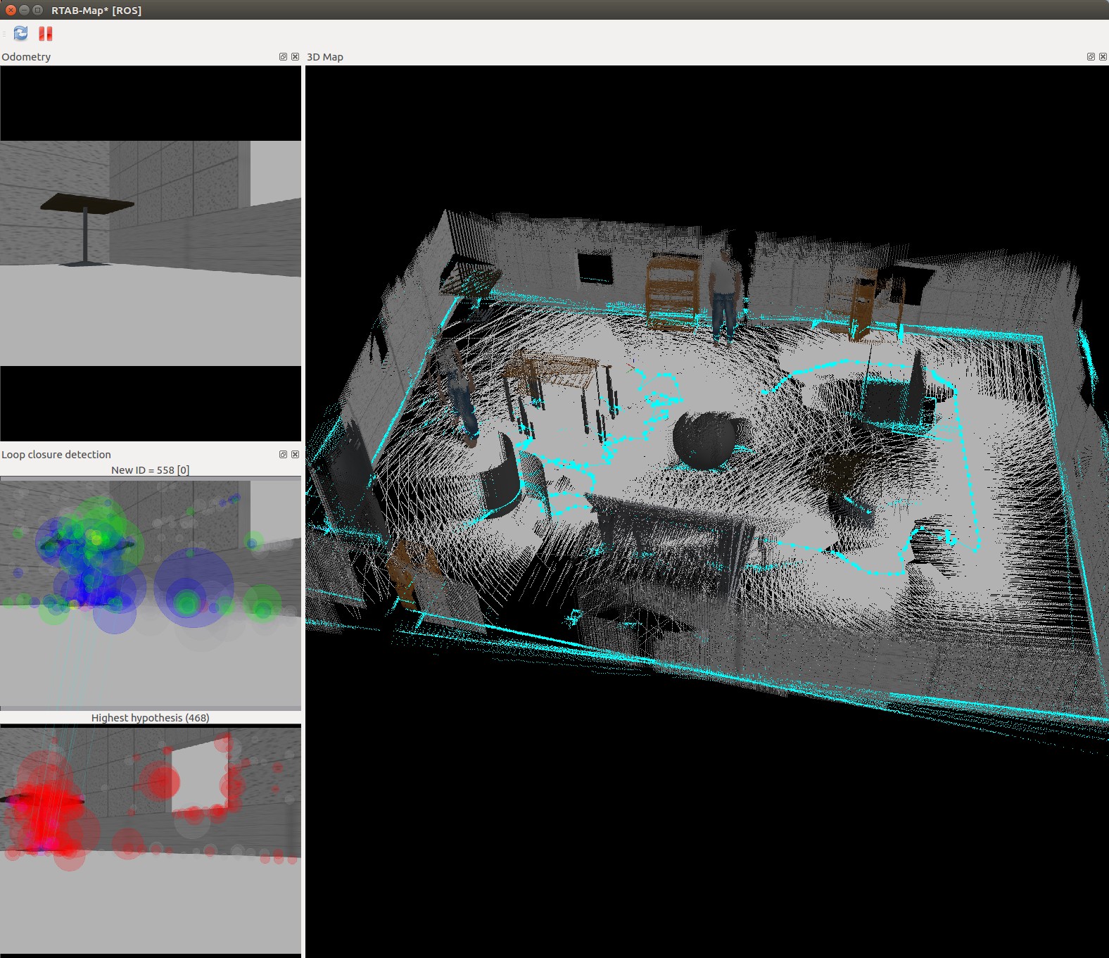
kitchen_dining_3d
kitchen_dining_2d
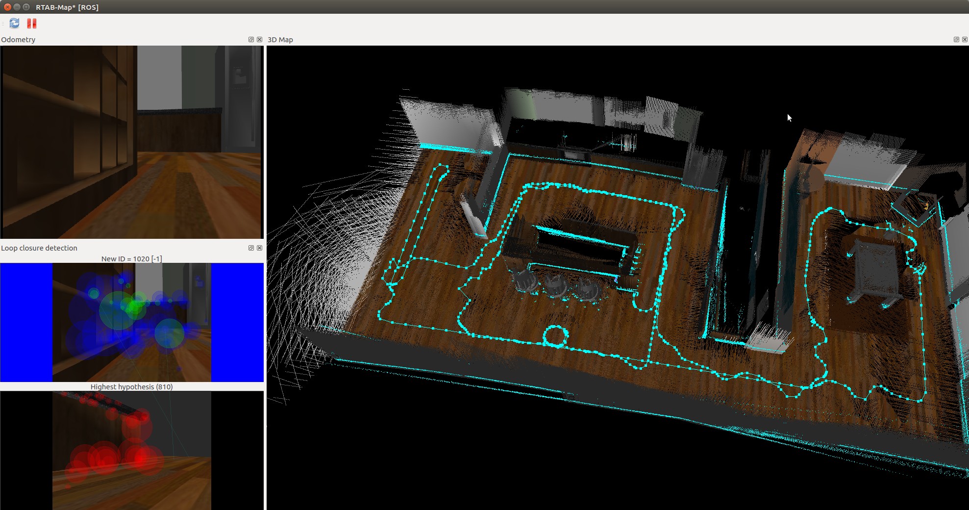
nicks_building_3d
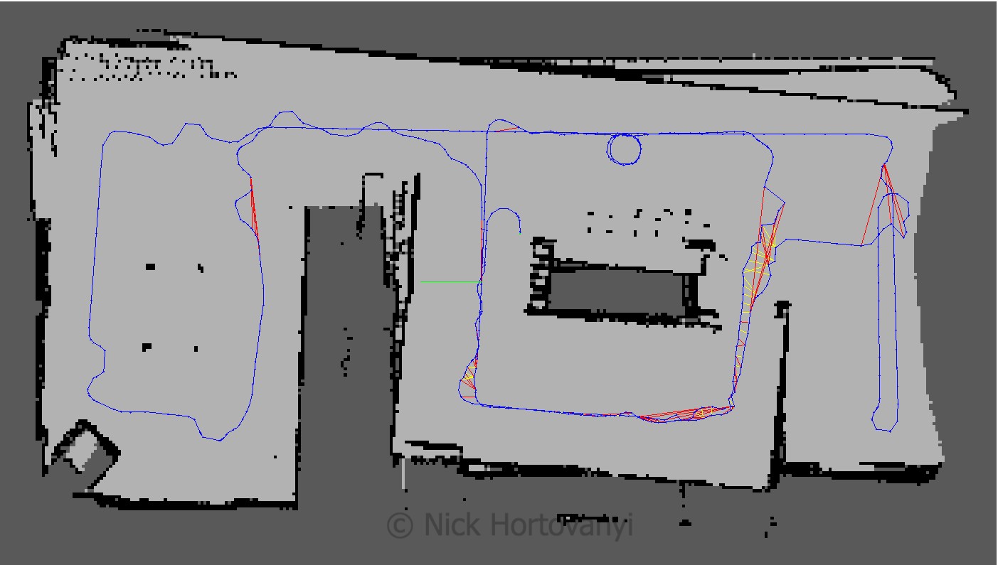
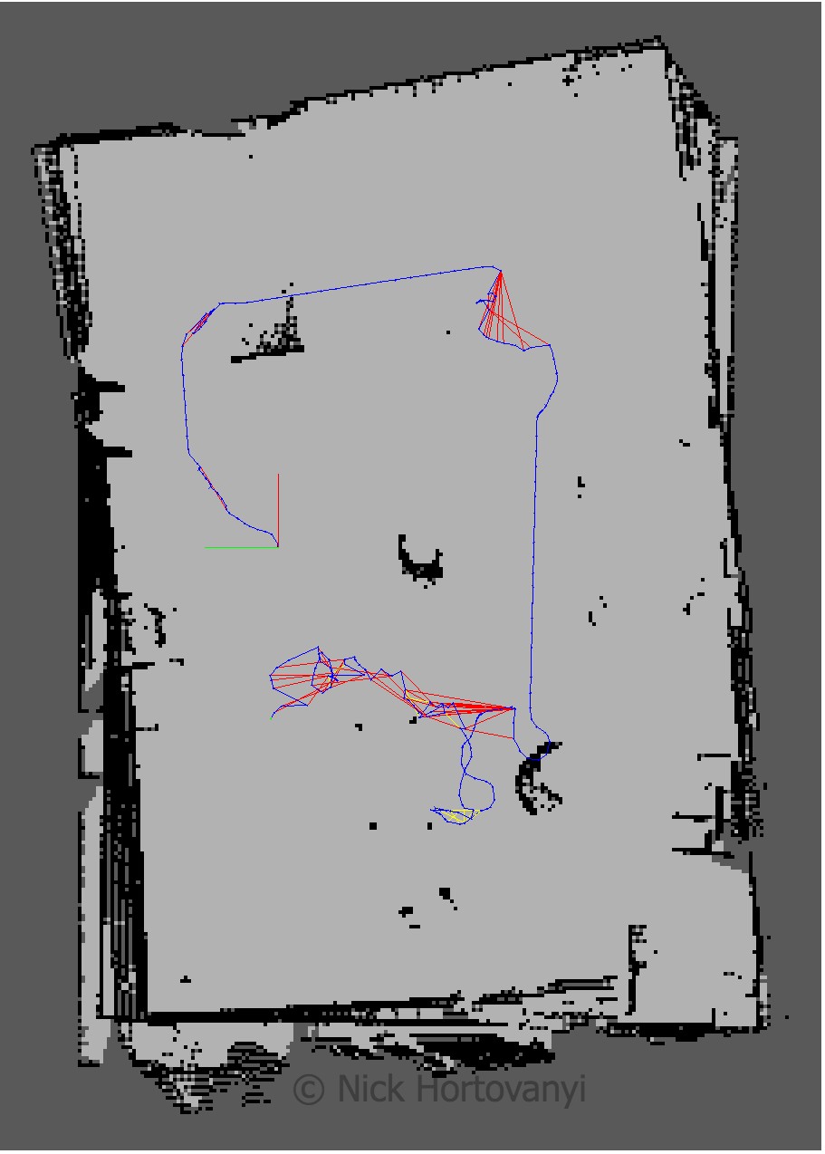
nicks_building_2d
Discusion
The robot was teleoped (navigated via the keyboard) around the room. At some points the robot did not move forward. This appeared to be when it started to perform loop closure. Kp/MaxFeatures was halved to 200 and Vis/MinInliers was reduced from 15 to 10.
However the 3D map quickly started to resemble the physical kitchen dining gazebo model. To improve loop detection rates some, on the spot circles were performed. Of particular note were the features in the main kitchen area. More SURF features were identified there as there was more variation in the surface s.
The nick building gazebo model wall surfaces were tiled, repeatable pattern with lack of other discerning features sometimes caused the loop closure detection to map to an incorrect previous image. This then distorted the map. Additional features were added to achieve a successful map.
The kitchen_dining model performed significantly better then the student created nicks_building model. This was due to the richer and more complex features of the kitchen_dining model.
Future Work
Mapping is important to help understand the world. There are a plethora of sensors and of interest is the about to arrive solid state lidars. As the price point of these sensors continues to drop it will open up opportunities to create richer and more realistic 3D maps at a cheaper price point.
Being able to map an environment cost effectively to create a replicated virtual world will increasingly be important to allow for the training of deep learning models. We are actively looking to do this and then supplant the trained model back into a robot so it can navigate in the original environment that was mapped.
The second project in term 2 of the Udacity Robotics Nano Degree program requires students to complete a hijacked robot scenario using ROS and Gazebo.
Students are to initially follow instructions for a building a reference robot model, before tuning the localisation parameters satisfactorily such that the robot within the Gazebo maze simulation can reach an end goal.
After completion of that, a new robot model is created with alterations to the base and position of sensors. Whereby it uses the same simulation and must reach the same end goal.
Introduction
In this project a robot model has to use localisation to work out where it is. It creates a rolling local map using laser range sensors. The local map in turn is used to navigate towards a navigation goal.
The navigation stack utilised move_base. It provides a local cost map, as the robot moves, in relation to a global cost map to define a continuous path for the robot to move along.
This project utilises Gazebo to create a simulation with a map provided by Clearpath Robotics
Once the robot has reached the navigation goal, the objective of the project has been achieved.
Background
A robot needs to understand where it is in a world, to be able to make navigation plans to get from point a, to point b, whilst avoiding obstacles. The process of understanding “where am I?” (from a robots perspective) is called localisation.
This project uses a localisation package built into ROS called Adaptive Monte Carlo Localisation (AMCL) to assist with the robot in a scenario to work out where it is. Hence the project name “Where am I?”.
AMCL is a variant of the Monte Carlo Localisation (MCL) which was learnt in the course material. MCL uses particles to localise the robot pose. It has several advantages over using Extended Kalman Filters (EKF) such as uses raw measurements (ie from lasers), is not reliant on gaussian noise, is memory and time efficient, and can perform global localisation.
The AMCL package adaptively alters the number of particles used, which has the advantage of reducing the computational overhead required.
Results
We first completed this exercise using the class room example which is named udacity_bot. Then a different version was created where the base and sensor locations were changed. This was named nick_bot and was launched using udacity_world_nick.launch.
The final results of when it reached the goal state follow.
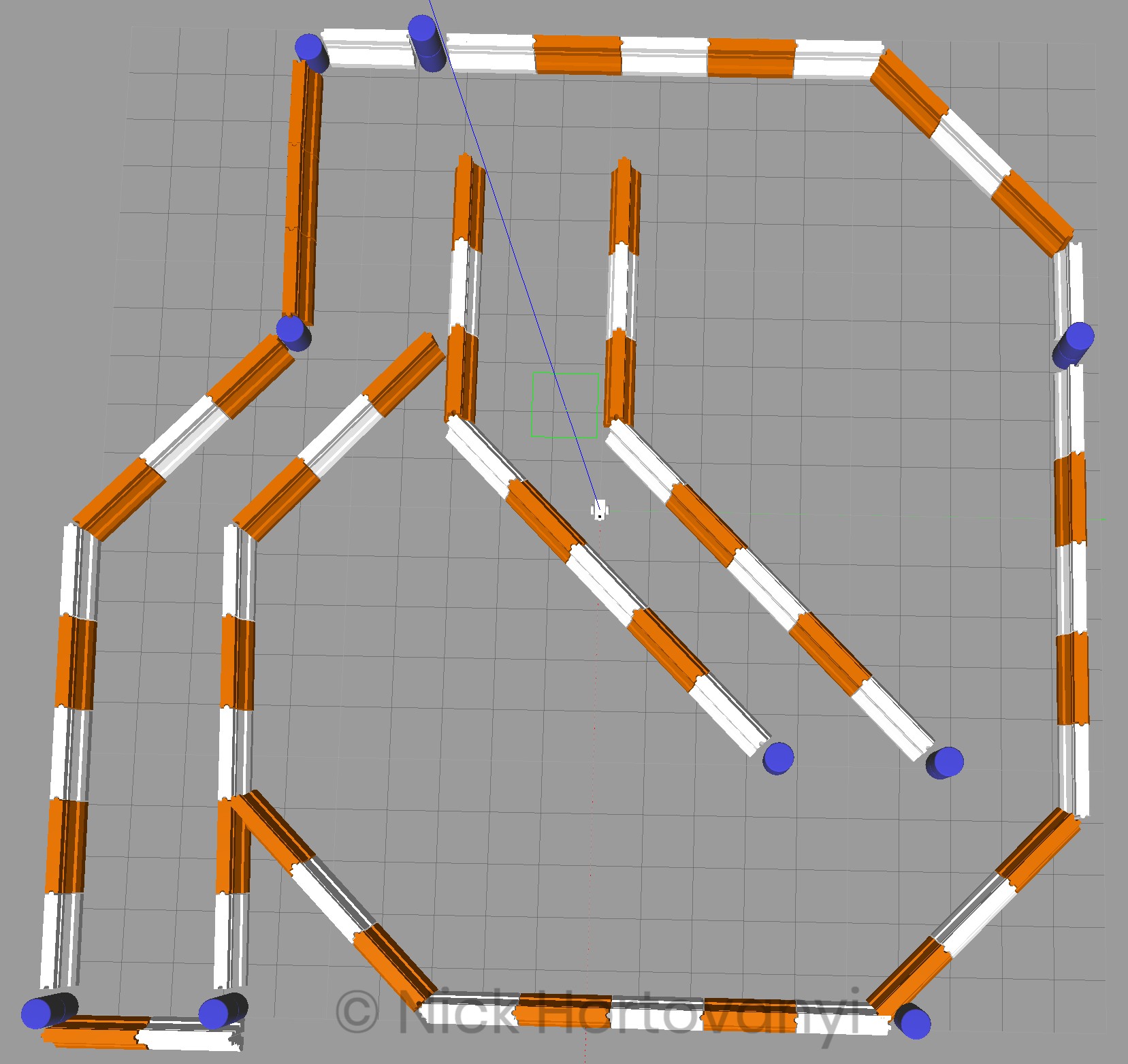
udacity_bot
udacity_bot rviz
nick_bot
nick_bot rviz
Model Configuration
This discussion is for the configuration of nick_bot.
The nick_bot was a square version of the rectangle based udacity_bot. The laser sensor was moved to the front of the robot.
The amcl_nick.lauch. Wherever possible the same configuration and parameters as the udacity_bot used amcl.launch.
min_particles was set to 25 and max_particles to 200 to not heavily utilise CPU. A higher max_particles did not improve initial ability of the robot to find itself with certainty.
odom_alpha1 to odom_alpha4 were trial & error values and changed from the default of 0.2 (there was not much documentation about).
The laser model parameters were left as default. There appeared no reason to change them as they were clearly visible on the above rviz visualisations and aligned to the barriers.
The yaw_goal_tolerance and xy_goal_tolerance were doubled from the default values to allow for additional flexibility in trajectory planning.
transform_tolerance was set 1.25 and update_frequency to 3.0 for both local and global.
obstacle_range was set to 1.5, raytrace_range to 4.0 and inflation_radius to 0.65 to enable sufficient space on the cost map for the robot to navigate.
robot_radius was set to 0.4 in this model to allow for the larger square design.
The local publish_frequency was set to 3.0 with the global to 5.0 This configuration in conjunction with 15.0 x 15.0 sized local cost map was able to function within the performance constraints of the system used. Increasing the size of the local cost map utilise significant more computer power and missed the time windows for publish_frequency.
sim_time was set to 4 as there appeared sufficient compute resource to estimate a trajectory out 4 seconds.
meter_scoring was enabled to ensure pdist_scale used meters.
pdist_scale was set to 0.5 being less than the default of 0.6. Default and higher values appeared to cause the robot to sometimes get stuck.
Discussion
The robot model was able to on most runs navigate successfully to the goal. The route taken at times could have been shortened. However further research is required into the ROS packages used to be able to tune it to achieve such. Often the observed path taken did not appear to be the most cost affective and when it missed the target goal, it would do a large sweep before re-approaching the target.
The AMCL routine appeared to quickly gain certainty about the locality of the robot. It was the rest of the navigation stack and move_base that needed further tuning.
In the kidnapped robot problem where by a robot is positioned in an arbitrary location, AMCL would be able to adapt the number of particles used to gain certainty of the robot’s location. In addition AMCL does not rely on landmarks, but on laser based maps, laser scans and transform messages to output pose estimates.
Moreover in an environment, where by there weren’t known landmarks, the AMCL has advantages over the Extended or Unscented Kalman Filter based approaches. These environments would include those with no known map (ie its the first time being navigated) or in highly unstructured environments with lots of moving structures over time eg shopping centres with popup shops in the aisles with significant foot traffic.
Future Work
The size of the local cost map had a significant impact on performance. Higher values decreased the ability to publish within the frequency required. In addition higher particle numbers whilst increasing CPU load did not reduce the time taken for the AMCL to be certain about the robots locality.
A square designed robot model as opposed to a rectangular design appeared to enable the robot to rotate more affectively around its base. Other wheel components are available but they did not publish ODOM information. Hence additional sensors might be required with further investigation into the impact of the removal of ODOM readings required.
A laser GPU gazebo component was available. This may enable reduced CPU load by moving the workload to the GPU.
A LIDAR unit would give a more complete map of the world around the robot. One could also look to include more laser sensors to map behind and to either side of the robot. This should facilitate with the creation of a more complete motion plan without the need for the robot to map it first.
When implementing this type of project on real hardware, the mobile nature of a robot, requiring it also to contain its own power sources, means that efficient usage of a CPU and GPU are a must. The higher the utilisation, the less effective time the robot will have to perform activities.
Thus whilst implementing more sensors may provide a more detailed and accurate map, in the field this would further drain the power source. Hence careful consideration is needed for the number of sensors, the total power consumption of the sensors and compute work loads, as well as the impact the quantity of data has to the compute utilisation rates whilst mobile.
If there no significant improvement in performance for the design objective and operational goals of the robot, then a more minimalist sensor and localisation cost map configuration may be appropriate.
The first project in term 2 of the Udacity Robotics Nano Degree program requires students to initiate their own inference project inclusive of data acquisition. The project builds on the initial reference project for digit image recognition inside the supplied Nvidia Digits environment.
The project ideas are the student’s own and must have at least 3 classification categories eg defective item vs normal item with classes (no item, defective item, normal item).
Introduction
Pedestrian and bicycle lanes are often crowded with many people not aware of or selectively ignoring the signage. It can lead, to an unsafe or hazardous environment, for all that use it with police officers reluctant to enforce the rules via fines.
The concept selected, in this project, was to classify an image as either containing a pedestrian, not-pedestrian or background.
The goal being, that some sought of visual representation via a screen with a smile or a frown, could be given to act, as a robotic traffic controller. Other potential instantiation could include a torso using upper body movement to signal good or bad behaviour.
Background / Formulation
During the initial inference task, on supplied data, GoogLeNet was chosen as it had a good inference rate per image with reasonable accuracy. Using the Adam Optimiser with an initial learning rate of .001, it was able to meet the numerical requirements of inference time below 10 ms with accuracy > 75%. The input used for this reference model in Nvidia’s DIGITS was 256×256 3 channel colour images.
Similar requirements of accuracy would be required for this inference project. It was not necessary to be a 100% accurate as a smiling or frowning face at least makes people think about what they are presently doing. It was not going to be used to issue fines or other enforcement notices. Video cameras would stream image data between 24-30fps which means that an Inception, VGG model and some ResNet models may be too slow for inference in real time.
With the additional perception that colour could also be useful in detecting pedestrian vs not-pedestrian, GoogLeNet was again chosen for this project using the Adam Optimiser with an initial learning rate of .001.
Other experimentation with using a higher initial learning rate of 0.01 with the above configuration over 5 epochs did not improve validation accuracy which remained around 50%. Similarly AlexNet over 5 epochs with the same Adam optimiser and learning rate did not increase accuracy. One experiment was performed using GoogLeNet with RMSProp optimiser and an initial learning rate 0.001 which did not result in improvement of validation accuracy but did have significantly higher training loss so was also not progressed.
Data Acquisition
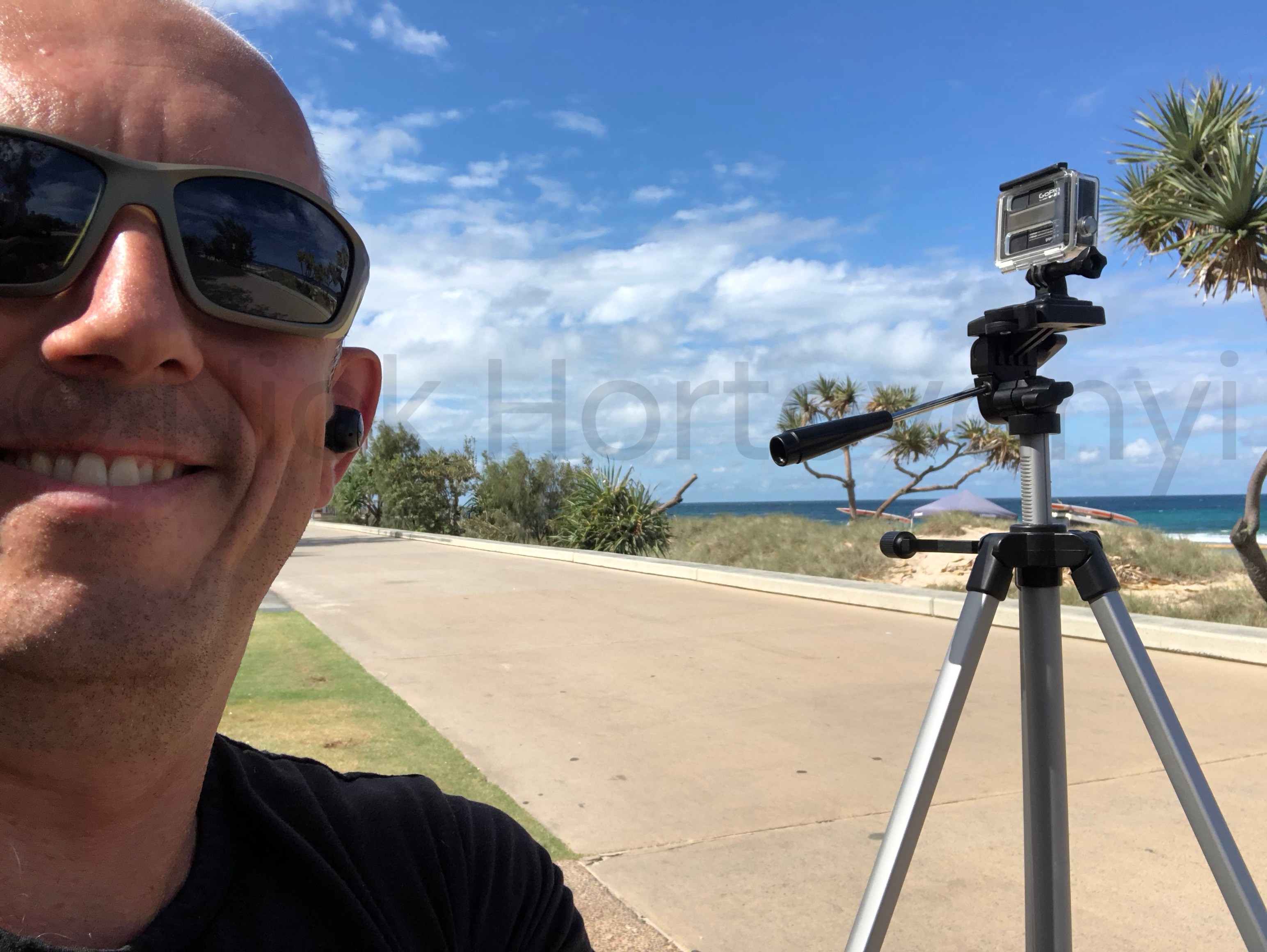
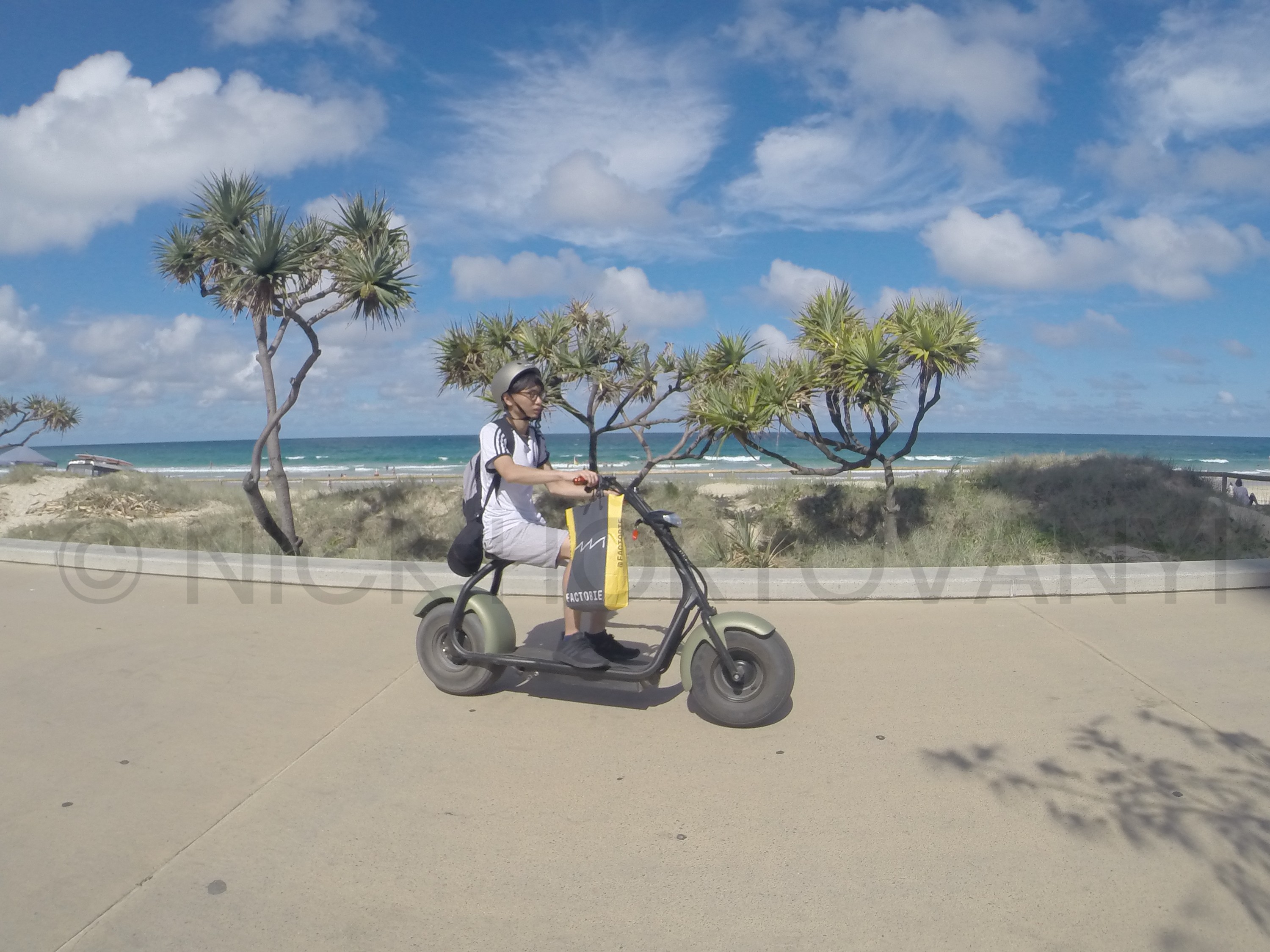
A GoPro mounted on a tripod was used. It was positioned on the side of a pedestrian esplanade at Surfers Paradise, Gold Coast, Australia. As it was summer holidays a reasonable amount of varying traffic was expected. The background looked over the ocean to have a consistent image where there was not going to be movement (besides cloud) other then what was on the esplanade.
GoPro Data Acquisition
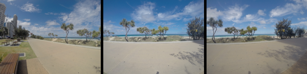
Three angles (facing left, centre and right) were used for capture per the following graphic:
Camera Background Angles
The GoPro was setup in wifi mode for time lapse capture, which was controlled via an iPhone. Initially 2 seconds elapsed was used, which eventually was dropped to 0.5. Using the GoPro time-lapse feature, meant that individual jpeg files were captured as opposed to a MP4 video.
Using the iPhone to control the control, meant that I could visualise what was coming before starting the next capture batch.
After the capture the images were manually placed into a directory for each category.
Image data was captured for the three categories background (322), pedestrian (349) and not-pedestrian (94). It became apparent at this time that not enough not-pedestrian image data had been captured. This was mainly due to the initial 2 seconds elapsed time used. Due to high heat and humidity of the Australian summer, in the following afternoons, it was not practical to capture more data from the same spot.
Skateboarders were placed in the pedestrian category.
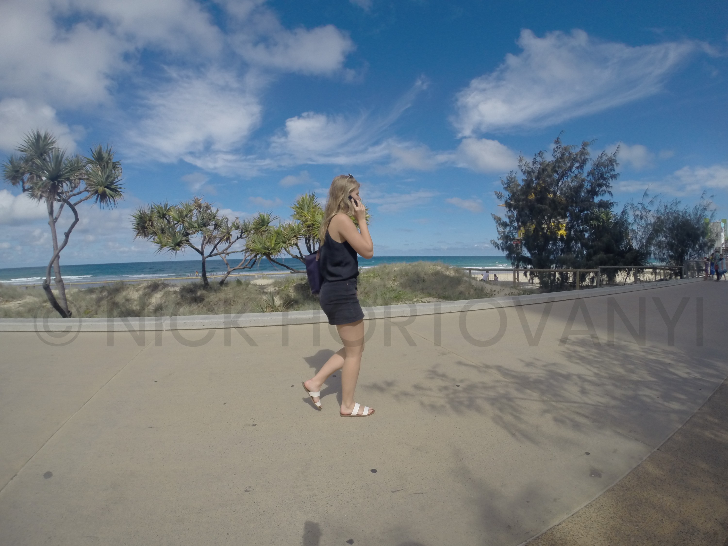
An example of a pedestrian and not-pedestrian follows. Background examples are as above.
not-pedestrian examplepedestrian example
A jupyter notebook was used to create a generator to supplement the data by randomising the image brightness, randomly flipping the images vertically and jittering the images randomly
in the x (by or – 25 pixels),y (by or – 50 pixels) planes to create supplemental image data.
The images were also resized to 256 x 256 and saved as PNGs.
The final generated supplemental data had 2000 not-pedestrian, 1000 pedestrian with 1000 background images.
Results
The initial inference task, on supplied data, GoogLeNet was chosen as it had a good inference rate per image with reasonable accuracy. Using the Adam Optimiser with an initial learning rate of .001, it was able to meet the numerical requirements of inference time below 10 ms (~5 ms actual) with accuracy > 75% (75.40984% actual).
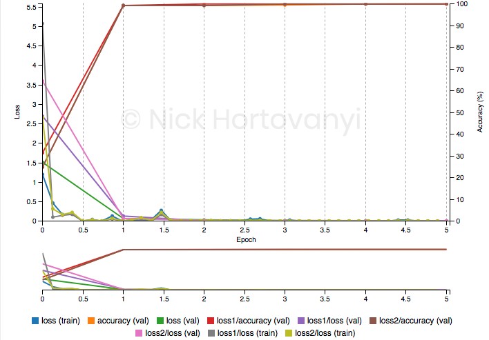
During training of the initial inference task 100% validation was achieved per the following training graph after 5 epochs.
Training Graph
However similar training results were not achieved for this inference project on captured data. The following training graph after 10 epochs follows
Project Training Graph
This had a validation accuracy of ~50%.
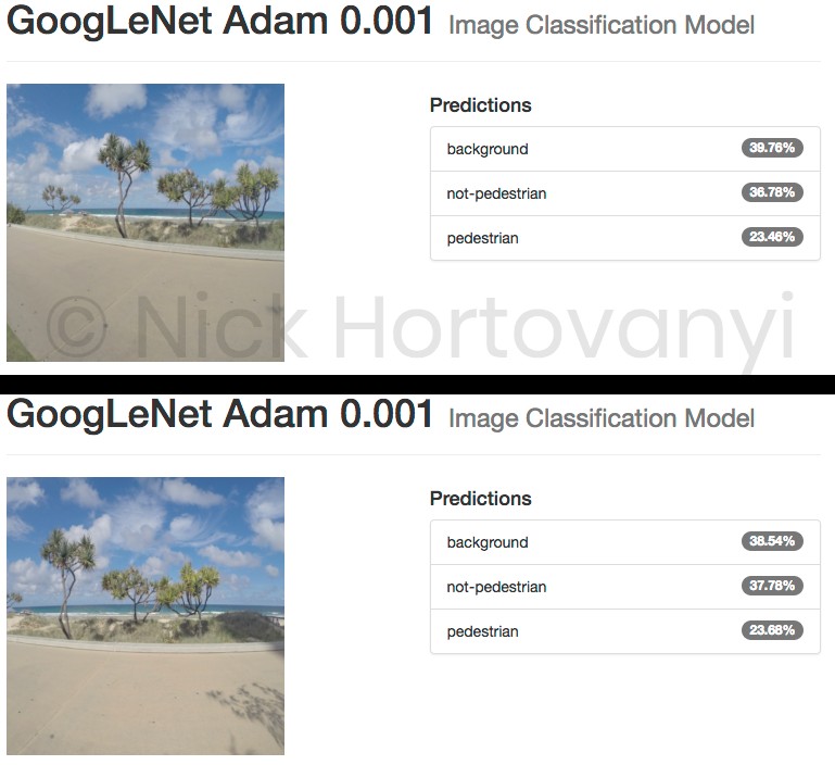
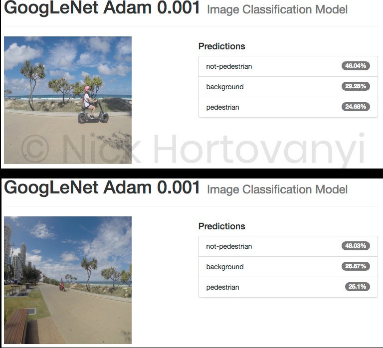
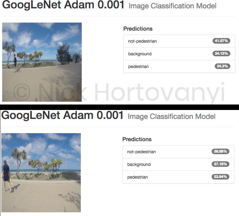
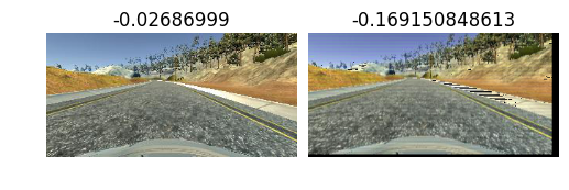
The following are the results of two randomly selected images per classification category uploaded as original high-res jpeg images from the GoPro.
The indicative inspection suggests that there was insufficient data to get a result > 75% for this project at this time. It also appears that the model as trained can not distinguish between pedestrian and not-pedestrian but can distinguish a background image.
Inference times were not tested separately as GoogLeNet is known to have a fast inference time which would be sufficient for this project.
Discussion
The dataset collected did not have enough sample images. This was as a result of using time-lapse with too high a value. In hind site, a combination of 0.5-1 sec time-lapse for slow moving pedestrians with >30 FPS video for higher speed moving non-pedestrians would of allowed for more data.
Of note is when there is a combination of non-pedestrian and pedestrian in the same frame led to the though of potentially using object detection first to find a window to classify. This was not implemented in this version however it would have led to a more accurate ability to classify as the background would be eliminated ie if no objects detected it must be a back ground image.
For this project the duration of a consistent display of say 2 to 3 seconds to the passing pedestrian and non-pedestrian traffic would drive the ultimate inference time required. It would suggest that it needs to be an average classification of a 1 second or two when leading up to where the video is captured.
Of note were skateboarders. There is only the skateboard (which has a low profile in the image) that distinguishes it from a pedestrian as velocity is not taken account with single images.
In addition the depth (away from the camera) of the traffic passing by changes the size of the object that needs to be classified. Pre-filtering and zooming these to a consistent size may improve accuracy.
Future Work
Whilst the project did not achieve a good train validation result, it has laid the foundation for future iterations. There is potential to capture more data and use object detection to refine the training and inference steps of the project.
Providing soft means to monitor and influence peoples decisions regarding signage and the associated rules for safe usage of (non-vehicle) transit paths would potentially be received positively by the community. Police forces lack the budget or people to enforce these rules and they are reluctant to issue minor infringement notices (with potential to destroy good will in the community). Hence a more subtle robotic person could improve the situation in a cost effective means.
The size of this market is unknown. However speed cameras using smiley and sad faces are used around the local area where I live. They are having a positive impact on driver behaviour in the areas deployed. Thus there is a market for a more community friendly and automated means to impact on behaviour.
Having completed, as one of the first, the Udacity Self Driving Car Nano Degree in October 2017, I thought I’d share some of the things I learnt along the way.
Rather than recap the projects, over the three terms, I’m going to focus in this post, on the philosophy and attitude I developed, to complete the nano degree program.
When I was first accepted, my initial reaction was geez have I bitten off more than I can chew. How am I going to cope with the mathematics and the theoretical side. It was a major concern.
Whilst at school I always had excelled at maths, and it was what led me initially into computing at a young age. I used to love writing graphics routines and optimising them. As my maths skills improved I learnt new ways of drawing circles and objects. I can’t remember if I got into Vectors. Yet past school, having started working in corporate IT, I had little use for maths skills besides that which was needed for Accounting. Yes for a number of years, IT dumbed down my maths skills.
IT was more focused on entering data, storing it and reporting on it at some monthly and yearly aggregate levels. Sure I worked on near realtime and mission critical systems but the need for very strong maths skills was limited. It was not a choice of my own, it was just that the technology that did leverage Maths, was perceived as scientific or too risky to adopt by business. It just didn’t have priority or urgency. Or if it was implemented it was a black box, that you supplied some input to, and you just consumed the output.
Getting back to the Self Driving Car Nano Degree, it was these black boxes that were our projects. In the project we needed to create the black boxes, to understand the theory and the mathematics.
Before starting the Nano Degree, I brushed up on matrices and vectors using the Kahn Academy.
Occasionally I got a little stuck on the mathematical proofs but once I understood the code for the maths, I normally was ok. Yes my brain now works off of code, not maths. We experienced some numerical instability, which was normally solved by interacting with others on the slack channels.
It was hard at times being the first going through the material. However with patience, with continuously reviewing the material, it reinforced what was being taught. You had to be methodical and test each assertion you were making about your code. Sometimes it required taking the algorithm and implementing in a repeatable test case inside a Jupyter Notebook. I found visualising the data improved understanding and helped to identify if anything was erroneous.
You could spend ages looking at the code and not see any obvious mistake. Without visualising the output, an easy mistake such as an incorrect sign in a rotation matrix, was not easy to observe.
The most valuable tool for when you got stuck was slack and your fellow students. These fellow students were online at all hours of the day, from across the globe.
After a few projects, I soon found an approach, that worked for me. It boiled down to learning, writing some code, seeing what happened, fixing what was broken, validating my learning and repeating until I had a project that met requirements.
Getting stuck, sometimes meant having a break, or having a late night. If I was really into tuning, it often meant the late night. Tweaking and trying different settings to get the Neural Network or Algorithm to achieve what you needed, was addictive. It was so much better, then reading or watching a video. The impact of changing your code was visible, in most projects in the simulator.
Your code didn’t produce a report, it produced observable action! It was like when I was a kid programming graphics for the first time.
So if your the type that likes to write those black boxes that other programmers use, you’ll excel at this Nano Degree. If your the type that consumes black boxes, that others have written, you may need to change your outlook.
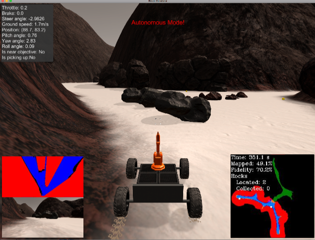
The goal of this project were to use perception and decision steps to control a rover in a simulator. Perception occurs via using computer vision techniques to determine navigable terrain and then make decisions to take Action on the rover.
Its the first project of the Robotics Nano Degree program. I ran my simulator in 1600×1200 resolution. Different resolution may impact on the performance of the model in this project.
Notebook Analysis
The first step was to perform some analysis in a jupyter notebook on sample/calibration data.
Run the functions provided in the notebook on test images (first with the test data provided, next on data you have recorded). Add/modify functions to allow for color selection of obstacles and rock samples.
This step involved loading the data
and then doing a perspective transform to get a birds eye view.
A function color_thresh was provided to do color thresholding (defaulted to RGB channels > 160). It was used as the basis to create an obstacle_thresh method (which selected the inverse ie RGB color channels <= 160). A rock_thresh method was created that selected between min and max color channels. The image color channels are converted from RGB to YUV before being used via warped_rock_yuv=cv2.cvtColor(warped_rock, cv2.COLOR_RGB2YUV).
Warped Threshed (white shows what is navigatable)Obstacle Threshed (white shows obstacle)Rock Threshed (white shows rock)
Populate the process_image() function with the appropriate analysis steps to map pixels identifying navigable terrain, obstacles and rock samples into a worldmap. Run process_image() on your test data using the moviepy functions provided to create video output of your result.
1) Define source and destination points for perspective transform
note: data.count contains the current position in index for the video stream.
6) Update worldmap (to be displayed on right side of screen)
for obstacle_x_world, obstacle_y_world in zip (xpix_world_obst, ypix_world_obst):
    data.worldmap[obstacle_y_world, obstacle_x_world, 0]  = 1
for rock_x_world, rock_y_world in zip (xpix_world_rock, ypix_world_rock):
    data.worldmap[rock_y_world, rock_x_world, 1]  = 1
for navigable_x_world, navigable_y_world, in zip(xpix_world, ypix_world):
    data.worldmap[navigable_y_world, navigable_x_world, 2]  = 1
7) Make a mosaic image
A mosaic image was created showing the rover camera image, warped image, ground truth (with rover location and direction arrow) and another ground truth (showing the current obstacle and navigable mapping)
Fill in the perception_step() (at the bottom of the perception.py script) and decision_step() (in decision.py) functions in the autonomous mapping scripts and an explanation is provided in the writeup of how and why these functions were modified as they were.
perception_step()
This step utilised the efforts from the notebook analysis, described above. The Rover Worldmap was not updated if there was observable pitch or roll (eg > or – 1 degree).
In addition rover polar coordinates were derived and saved against the passed Rover object for both navigable areas and observed rocks (if no rocks observed set to None).
decision_step()
This is the challenging part of the project.
stop and forward were the two default rover modes supplied. For this project stuck, rock and reverse were added.
forward was modified to have a left hugging biases by adding 65% of the standard deviation of the navigable angles, as long as there had been some travel time either initially or after being stuck.
The rover enters stuck mode if the rover stays in the same position, whilst not picking up a rock, for 5 seconds. If still stuck after 10 seconds, then reverse mode is tried. After 15 seconds, stuck and reverse are reset before trying stop mode.
stuck mode tries rotating if there is an obstruction in front, moving forward if steering not locked full left or right whilst going slow, and breaking if steering is locked full left or right. It will reset to forward if movement is restored.
reverse mode rotates randomly between 30 and 180 degrees after setting the brakes and reducing velocity to zero. Once its within or – 15 degrees it sets mode to forward. If reverse mode is in-affective to sets it to stop mode.
If a rock is observed, some false positives are ignored, as well as distant rocks before being placed into rock mode. Whilst the rock is not close, it tries to navigate closer towards it before breaking or coasting closer. The algorithm still requires more refinement.
Note: All my testing and running in Autonomous mode was done at 1600×1200 resolution.
This MPC (Model Predictive Controller) project, was the last in term 2 of the Udacity Self Driving Car Engineer Nanodegree.
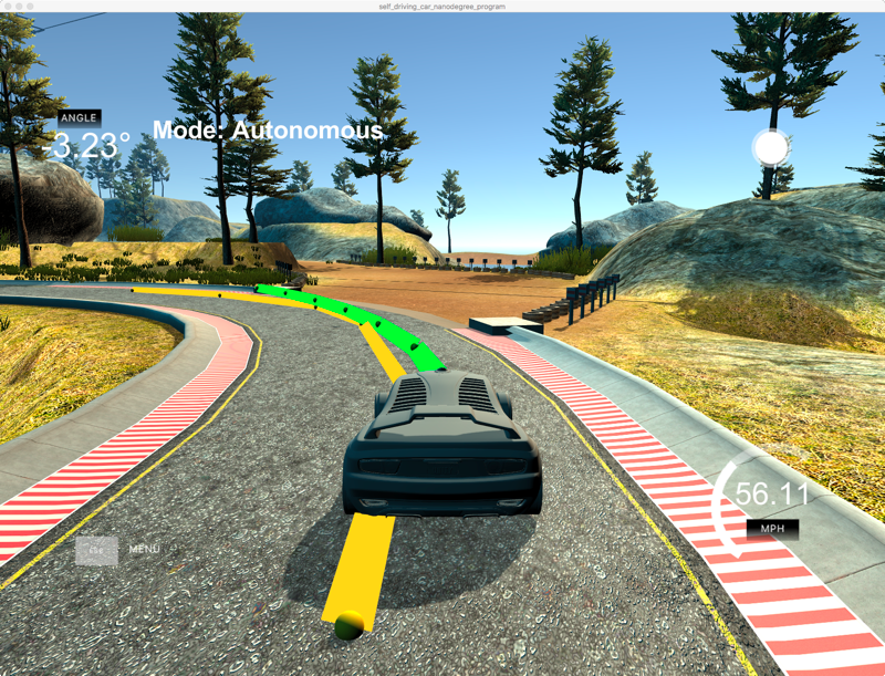
Simulator output
This MPC (Model Predictive Controller) project, was the last in term 2 of the Udacity Self Driving Car Engineer Nanodegree.
Implementation
The Model
For this project (github repo) we used a global kinematic model, which is a simplification of a dynamic model that ignores tire forces, gravity and mass.
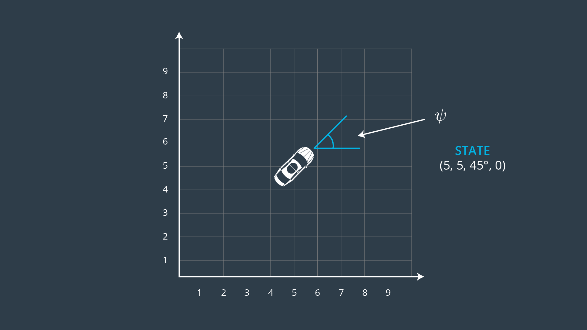
The state model is represented by the vehicles position, orientation angle (in radians) and velocity.
A cross track error (distance of vehicle from trajectory) and an orientation error (difference of vehicle orientation and trajectory orientation) were also included in the state model.
Two actuators were used, delta – to represent the steering angle (normalised to [-1,1]) and a – for acceleration corresponding to a throttle, with negative values for braking.
The simulator passes via a socket, ptsx & ptsy of six waypoints (5 in front, 1 near the vehicle), the vehicle x,y map position, orientation and speed (mph).
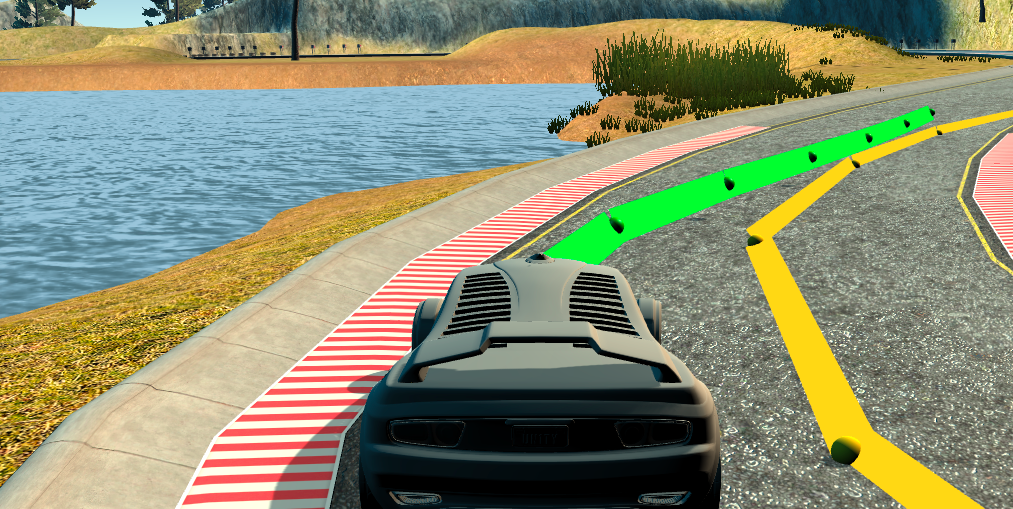
This data after being transformed into the vehicle map space, with new cross track error and orientation error calculated, is then passed into the MPC (Model Predictive Control) solve routine. It returns, the two new actuator values, with steering and acceleration (i.e. throttle) and the MPC predicted path (plotted in green in the simulator).
Constraint costs were applied to help the optimiser select an optimal update. Emphasis was placed on minimising orientation error and actuations, in particular steering (to keep the lines smooth).
   // Reference State Cost
    // TODO: Define the cost related the reference state and
    // any anything you think may be beneficial.
    // The part of the cost based on the reference state.
    for (int i = 0; i < N; i  ) {
      fg[0]  = CppAD::pow(vars[cte_start   i] - ref_cte, 2);
      fg[0]  = 2 * CppAD::pow(vars[epsi_start   i] - ref_epsi, 2);
      fg[0]  = CppAD::pow(vars[v_start   i] - ref_v, 2);
    }

    //
    // Setup Constraints
    //
    // NOTE: In this section you'll setup the model constraints.
    // Minimize the use of actuators.
    for (int i = 0; i < N - 1; i  ) {
      fg[0]  = CppAD::pow(vars[delta_start   i], 2);
      fg[0]  = CppAD::pow(vars[a_start   i], 2);
    }

    // Minimize the value gap between sequential actuations.
    for (int i = 0; i < N - 2; i  ) {
      fg[0]  = 20000 * CppAD::pow(vars[delta_start   i   1] - vars[delta_start   i], 2);
      fg[0]  = 10 * CppAD::pow(vars[a_start   i   1] - vars[a_start   i], 2);
    }
Timestep Length and Frequency
The MPC optimiser has two variables to represent the horizon into the future to predict actuator changes. They are determined by N (Number of timesteps) and dt (timestep duration) where T (time) = N * dt.
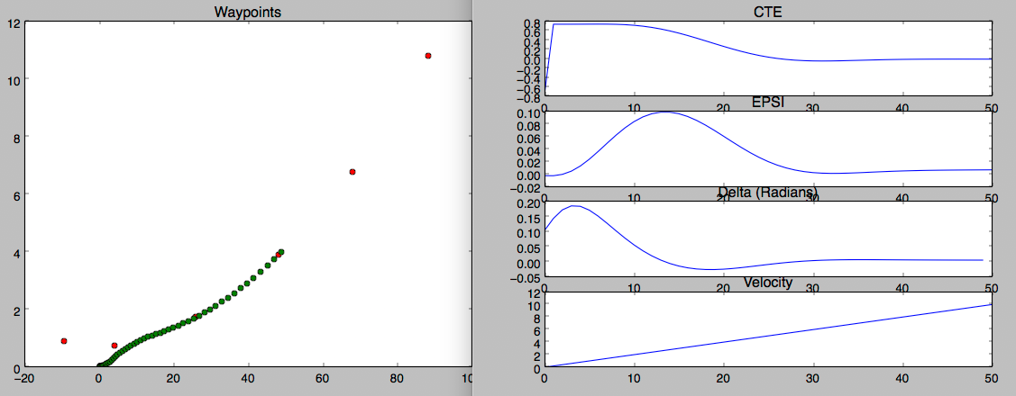
To help tune these settings, I copied the mpc_to_line project quiz, to a new project mpc_to_waypoint, and modified it to represent the initial state model to be used with the Udacity simulator. I was able to get good results looking out 3 seconds, with N = 15 and dt = 0.2. The following output are plots of 50 iterations from the initial vehicle state:
It seemed to be tracking quite nicely but speed was very slow.
However what I found, is that a horizon out 3 seconds in the simulator seemed to be too far. The faster the vehicle, the further forward the optimiser was looking. It shortly started to fail and the vehicle would end up in the lake or even worse airborne.
I tried reducing N and increasing dt. Eventually, via trial and error, I found good results where N was 8 to 10 and dt between ~0.08 to ~0.105. I eventually settled on calculating dt based on Time/N (with time set at ~.65 seconds and N on 8). If I saw the plotted MPC line coming close to the 2nd furthest plotted waypoint at higher speeds, it started to correspond, with the MPC optimiser failing.
The reference speed also played a part. To drive safely around the track, to ensure the project meets requirement, I kept it at 60 MPH.
Polynomial Fitting and MPC Preprocessing
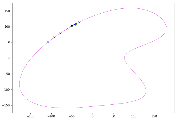
An example plot of the track with the first way points, vehicle position and orientation follows:
To make updating easier and to provide data to be able to draw, the waypoints and the predicted path from the MPC solver, coordinates were transformed into vehicle space. This meant also that the initial position of the vehicle state, for the solver was (0 velocity in KPH * 100 ms of latency,0), which included a projection of distance travelled to cover latency, with a corresponding angle orientation of zero. These coordinates were used in the poly fit. It had an added benefit of simplifying, the derivative calculation required for the orientation error.
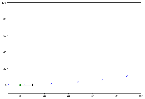
The following plot is the same waypoints transformed to the vehicle space map, with the arrow representing the orientation of the vehicle:
Model Predictive Control with Latency
Before sending the result back to the simulator a 100ms latency delay was implemented.
this_thread::sleep_for(chrono::milliseconds(100));
This replicated the actuation delay that would be experienced in a real-world vehicle.
I experimented with trying to understand if the ratio of dt (time interval) to latency in seconds, being near 1 (i.e. the time interval was close to the latency value), had an impact on the ability of the MPC algorithm to handle latency. Anecdotal evidence supported that; but in reality ratio values of < 1 (for this project, I had (.65/8)/.100 = .0.8125) were the reality to ensure the optimiser was able to find a solution.
As described in the previous section, the vehicle position was projected forward, the distance it would travel, to cover 100ms of latency.
However before I implemented the forward projection for latency, you could see in places where the vehicle lagged a little in its turning. The MPC, however predicted the path correctly back onto the centre line of the track per following image:
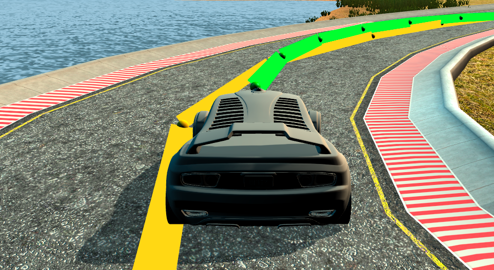
After I implemented the latency projection calculation, the vehicle was able to stay closer to center, more readily per this image:
Over all the drive around this simulator track, was smoother and lacked steering wobbles, when compared to using a PID controller.
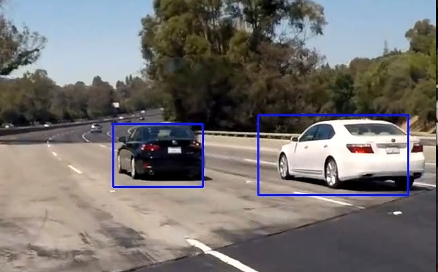
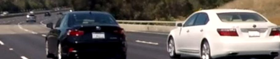
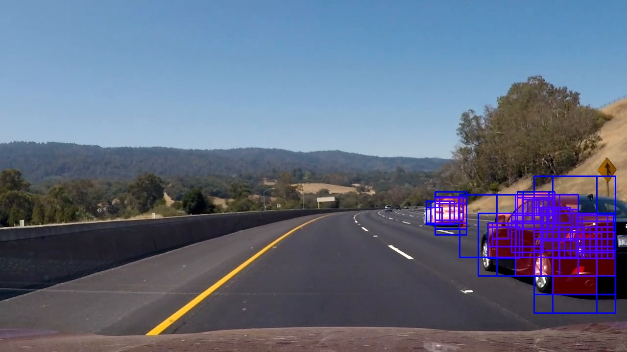
In this vehicle detection and tracking project, we detect in a video pipeline, potential boxes, via a sliding window, that may contain a vehicle by using a Support Vector Machine Classifier for prediction to create a heat map. The heat map history is then used to filter out false positives before identification of vehicles by drawing a bounding box around it.
Vehicle Detection Sample
Vehicle Detection Project
The goals / steps of this project are the following:
Perform a Histogram of Oriented Gradients (HOG) feature extraction on a labeled training set of images and train a classifier Linear SVM classifier
Optionally, you can also apply a color transform and append binned color features, as well as histograms of color, to your HOG feature vector.
Note: for those first two steps don’t forget to normalize your features and randomize a selection for training and testing.
Implement a sliding-window technique and use your trained classifier to search for vehicles in images.
Run your pipeline on a video stream (start with the test_video.mp4 and later implement on full project_video.mp4) and create a heat map of recurring detections frame by frame to reject outliers and follow detected vehicles.
Estimate a bounding box for vehicles detected.
A jupyter/iPython data science notebook was used and can be found on github Full Project Repo – Vehicle Detection Project Notebook (Note the interactive ipywidgets are not functional on github). As the notebook got rather large I extracted some code into python files utils.py (functions to extract, loading helpers), features.py (feature extraction and classes), images.py (image and window slice processing), search.py (holds search parameters class), boxes.py (windowing and box classes) and detection.py (main VehicleDetection class that coordinates processing of images). The project is written in python and utilises numpy, OpenCV, scikit learn and MoviePy.
Histogram of Oriented Gradients (HOG)
Through a bit of trial and error I found a set of HOG parameters.
HOG Feature Extraction and Parameters
A function extract_hog_features was created that took an array of 64x64x3 images and returned a set of features. These are extracted in parallel and it in turn uses HogImageFeatures class.
As the hog algorithm is primarily focused on grey images, I initially used the YCrCB colour space with the Y channel (used to represent a gray images). However I found that it was not selective enough during the detection phase. I thus used all 3 colour channels. To reduce the number of features, I increased the number of HOG pixels per cell. I used an interactive feature in my notebook to find an orient setting of 32 that showed distinctive features of vehicle. Sample follows.
Training Vehicle HOG Sample
The final parameter settings used color_space = 'YCrCb',orient = 32,pix_per_cell = 16 and hog_channel = 'ALL'. Experimentation occurred with using Colour Histogram Features but it slowed down feature extraction and later increased the number of false positives detected. Per the following visualisation graphic, you can see that the Cr and Cb colour spaces had detectable hog features
Sample HOG Channel Output form a video window slice
Classifier Training
Once HOG features (no Colour Hist or Bin Spatial) were extracted from car (GTI Vehicle Image Database and Udacity Extras) and not_car (GTI, KITTI) image sets. They were then stacked and converted to float in the vehicle detection notebook.
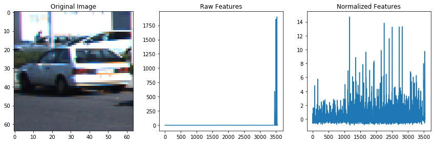
Features were then scaled using the Sklearn RobustScaler sample result follows.
Experimentation occurred in the Classifier Experimentation Notebook between LinearSVC (Support Vector Machine Classifier), RandomForest and ExtraTrees classifiers. LinearSVC was chosen as the prediction time was 0.00228 seconds for 10 labels compared to ~0.10 seconds for the other two.
Sliding Window Search
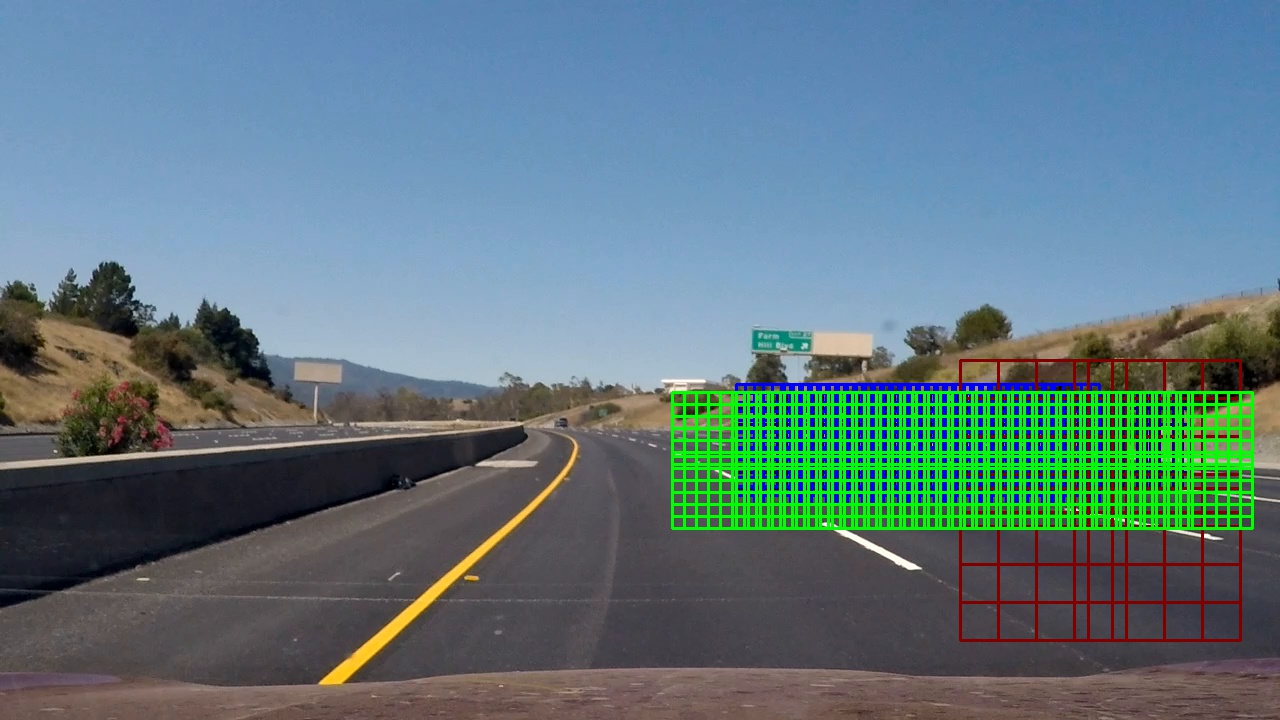
Building sliding windows
For this project four sizes of windows were chosen – 32×32, 48×48, 64×64 and 128×128 and position at different depth perspective on the bottom right side of the image to cover the road. The larger windows closer to the driver and the smaller closer to the horizon. Overlap in both x,y was set between 0.5 and 0.8 to balance the need for better coverage vs number of boxes generated – currently 937. The more boxes for a sliding window, the more calculations per video image.
Classifier examples and optimisation
Some time was spent on parallelisation of the search using Python async methods and asyncio.gather in the VehicleDetection class. The search extracts the bounded box image of each sized search window and scales it to 64×64 before doing feature extraction and prediction on each window.
The search hot_box_search returns an array of hot boxes that classifier has predicted contains a vehicle.
These boxes overlap and are used to create a clipped at 255, two dimensional heat map. To remove initial false positives counts > 4 are kept. The heat map is then normalised before another threshold is applied
A history is kept of heat maps which is then used as input into Scipy Label with a dim binary structure linking dimensions, giving
finally a variance filter is applied on each box, if for one detected label boxes are ignored with a variance < 0.1 (its just a few close points0 or if multiple with a variance < 1.5 (more noise).
One of the nice features of the scipy.ndimage.measurements.label function is that it can process 3d arrays giving labels in x,y,z spaces. Thus when using the array of heat map history as input, it labels connections in x,y,z. If a returned label box is not represented in at least 3 (heat map history max – 2) z planes then it is rejected as a false positive. The result is that a vehicle is tracked over the heat map history kept.
Discussion
When construction this pipeline, I spent some time working on parallelising the window search. What I found is that there is most likely little overall performance improvement to be gained by doing so. Images have to be processed in series and whilst generating the video, my cpu was under utilised.
In hindsight I should of used a heavy weight search to detect vehicles and then a more lighter weight, narrower search primed by the last known positions. Heavy weight searching could be run at larger intervals or when a vehicle detection is lost.
My pipeline would fail presently if vehicles were on the left hand side or centre of the car. I suspect trucks, motorbikes, cyclists and pedestrians would not be detected (as they are not in the training data).
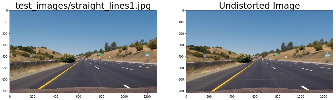
In this Advanced Lane Detection project, we apply computer vision techniques to augment video output with a detected road lane, road radius curvature and road centre offset. The video was supplied by Udacity and captured using the middle camera.
sample lane detection result
The goals / steps of this project are the following:
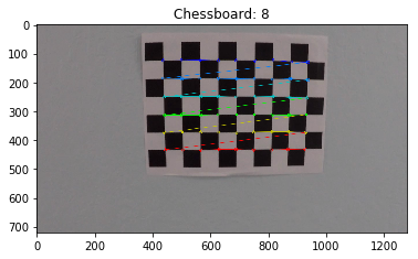
Compute the camera calibration matrix and distortion coefficients given a set of chessboard images.
Apply a distortion correction to raw images.
Use color transforms, gradients, etc., to create a thresholded binary image.
Apply a perspective transform to rectify binary image (“birds-eye view”).
Detect lane pixels and fit to find the lane boundary.
Determine the curvature of the lane and vehicle position with respect to center.
Warp the detected lane boundaries back onto the original image.
Output visual display of the lane boundaries and numerical estimation of lane curvature and vehicle position.
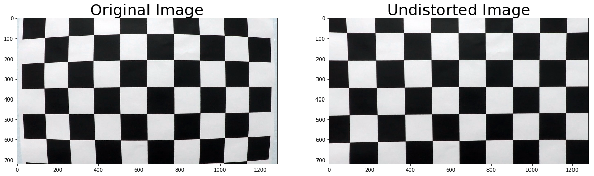
Every camera has some distortion factor in its lens. The known approach to correct for that in (x,y,z) space is apply coefficients to undistort the image. To calculate this a camera calibration process is required.
It involves reading a set of warped chessboard images, converting them into grey scale images before using cv2.findChessboardCorners() to identify the corners as imgpoints.
If corners are detected then they are collected as image points imgpoints along with a set of object points objpoints; with an assumption made that the chessboard is fixed on the (x,y) plane at z=0 (object points will hence be the same for each calibration image).
In the function camera_calibrate I pass the collected objpoints, imgpoints and a test image for the camera image dimensions. It in turn uses cv2.calibrateCamera() to calculate the distortion coefficients before the test image is undistorted with cv2.undistort() giving the following result.
Pipeline (Test images)
After camera calibration a set of functions have been created to work on test images before later being used in a video pipeline.
Distortion corrected image
The undistort_image takes an image and defaults the mtx and dist variables from the previous camera calibration before returning the undistorted image.
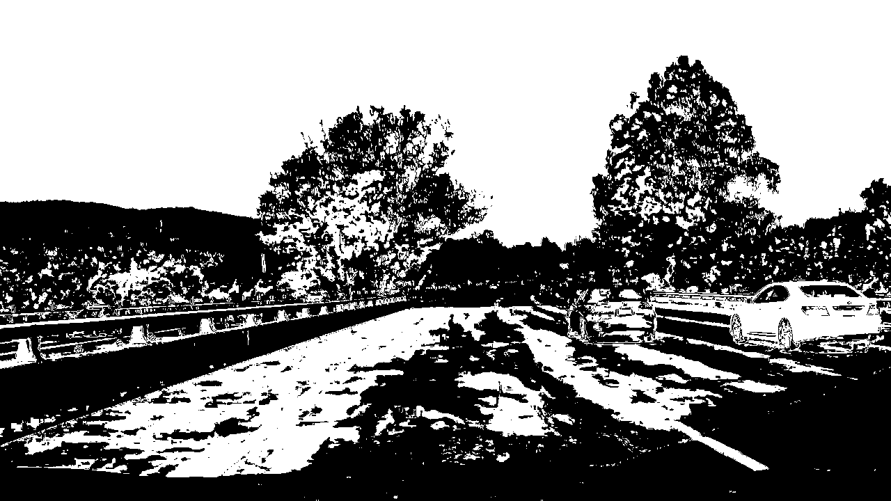
Threshold binary images
A threshold binary image, as the name infers, contains a representation of the original image but in binary 0,1 as opposed to a BGR (Blue, Green, Red) colour spectrum. The threshold part means that say the Red colour channel( with a range of 0-255) was between a threshold value range of 170-255, that it would be set to 1.
A sample output follows.
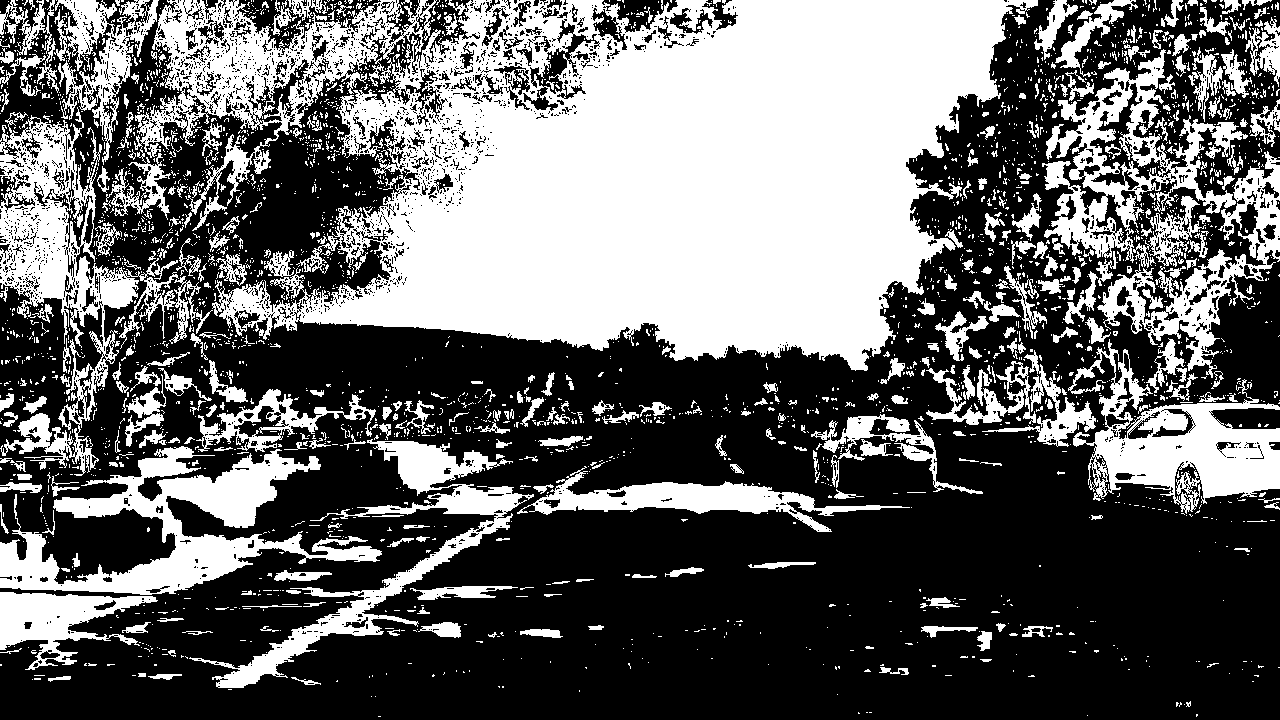
Initial experimentation occurred in a separate notebook before being refactored back into the project notebook in the combined_threshold function. It has a number of default thresholds for sobel gradient x&y, sobel magnitude, sober direction, Saturation (from HLS), Red (from RGB) and Y (luminance from YUV) plus a threshold type parameter (daytime-normal, daytime-bright, daytime-shadow, daytime-filter-pavement).
Whilst the daytime-normal threshold worked great for the majority of images there were situations where it didn’t e.g. pavement colour changes in bright light and shadow.
Daytime Normal with noise bright light & pavement changeDaytime Normal with shadow
To be able to detect the road lines, the undistorted image is warped. The function calc_warp_points takes an image’s height & width and then calculates the src and dst array of points. perspective_transforms takes them and returns two matrixes M and Minv for perspective_warp and perpective_unwarp functions respectively. The following image, shows an undistorted image, with the src points drawn with the corresponding warped image (the goal here was straight lines)
Lane-line pixel identification and polynomial fit
Once we have a birds eye view with a combined threshold we are in a position to identify lines and a polynomial to draw a line (or to search for points in a binary image).
topdown warped binary image
A histogram is created via lane_histogram from the bottom third of the topdown warped binary image. Within lane_peaks, scipy.signal is used to identify left and right peaks. If just one peak then the max bin either side of centre is returned.
calc_lane_windows uses these peaks along with a binary image to initialise a left and right instance of a WindowBox class. find_lane_window then controls the WindowBox search up the image to return an array of WindowBoxes that should contain the lane line. calc_fit_from_boxes returns a polynomial or None if nothing found.
poly_fitx function takes a fity where fity = np.linspace(0, height-1, height) and a polynomial to calculate an array of x values.
The search result is plotted on the bottom left of the below image with each box in green. To test line searching by polynomial, I then use the left & right WindowBox search polynomials as input to calc_lr_fit_from_polys. The bottom right graphic has the new polynomial line draw with a blue search window (relates to polynomial used for the search from WindBoxes) that was used overlapping with a green window for the new.
Warped box seek and new polynomial fit
Radius of curvature calculation and vehicle from centre offset
In road design, curvature is important and its normally measured by its radius length. For a straight line road, that value can be quite high.
In this project our images are in pixel space and need to be converted into meters. The images are of US roads and I measured from this image the distance between lines (413 pix) and the height of dashes (275 px). Lane width in the US is ~ 3.7 meters and dashed lines 3 metres. Thus xm_per_pix = 3.7/413 and ym_per_pix = 3./275 were used in calc_curvature. The function converted the polynomial from pixel space into a polynomial in meters.
To calculate the offset from centre, I first determined where on the x plane, both the left lx and right rx lines crossed the image near the driver. I then calculated the xcentre of the image as the width/2. The offset was calculated such (rx - xcenter) - (xcenter - lx) before being multiple by xm_per_pix.
Final pipeline
I decided to take a more python class based approach once I progressed through this project. Inside the classes, I called the functions mentioned previously. The classes created were:
Lane contains image processing, final calculations for view drawing and reference to left and right RoadLines. It also handled searching for initial lines, recalculations and reprocessing a line that was not sane;
RoadLine contains a history of Lines and associated curvature and plotting calculations using weighted means; and
Line contains detailed about the line and helper functions
Processing is triggered by setting the Lane.image variable. Convenient property methods Lane.warped, Lane.warped_decorated, lane.result and lane.result_decorated return processed images. It made it very easy to debug output using interactive ipywidgets (which don’t work on github)
To some degree, I got distracted with trying to solve the issues I found in my algorithm with the challenge videos. This highlighted, that I need to improve my understanding of colour spaces, sobel and threshold combinations.
I included a basic algorithm to remove pavement colours from the images using a centre, left and right focal point. I noticed that the dust colour on the vehicle seemed to be also in the road side foliage. This however wasn’t sufficient to remove all pavement colour and didn’t work when there was a road type transition. It was very CPU intensive.
In the end, I used a combination of different methods, that used a basic noise filter on warped binary images to determine, if it was sufficient to look for a line or not. If it wasn’t it tried the next one, with the final being a vertical rectangle window crawl down the image. Where the best filter was determined for each box. Again this was CPU intensive, but worked.
Another issue faced was using the previous curvature radius to determine if this line was sane or not. The values were too jittery and when driving on a straight line, high. I decided not to pursue this.
Opportunities for improvement in the algorithm/pipeline
There is room here for some refactoring into a more Object oriented approach. This was not evident at the start of the project as to how it should be structured. I experimented a little with using Pool from multiprocessing to parallelise left and right lane searches. It didn’t make it into my final classes as for normal line searching using a polynomial, as I did not ascertain if the multiprocessing overhead, outweighed the parallelism value. Certainly potential here to use a more functional approach to give the best runtime options for parallelisation.
Other areas, include automatically detecting the src points for warp, handling bounce in the road and understanding surface height (above road) of the camera and its impact.
I thought also as I’ve kept history, I could extend the warp to include a bird’e eye representation of the car on the road and directly behind it. I did mean averaging on results for smoothing drawn lines, but this was not included in the new line calculations from the next image frames.
The algorithm could also be made to make predictions about the line when there is gaps. This would be easier with continuous lines then dashed.
Hypothetical pipeline failure cases
Pavement fixes and/or combined with other surfaces that create vertical lines near existing road lines.
It would also fail if there was a road crossing or a need to cross lanes or to exit the freeway.
Rain and snow would also have an impact and I’m not sure about night time.
Tail gating a car or a car on a tighter curve would potentially interrupt the visible camera and hence line detection.
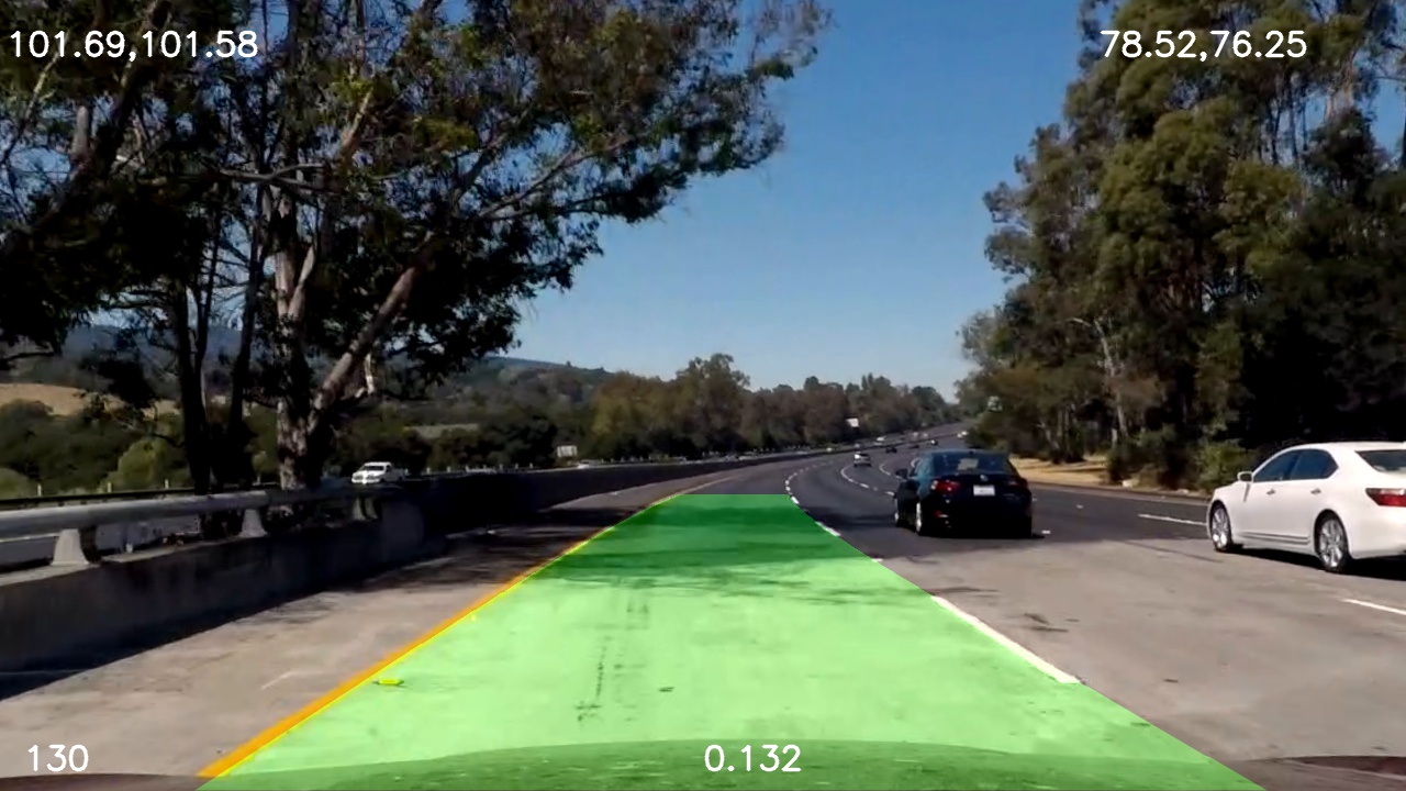
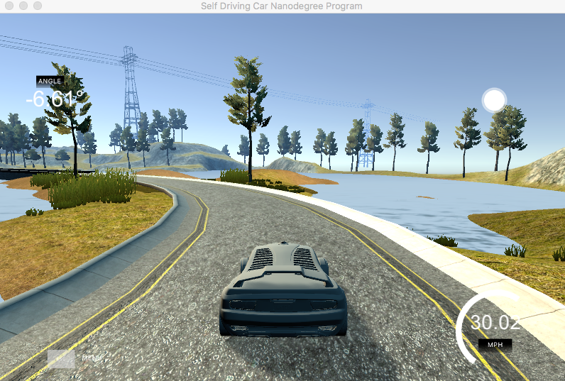
With this behaviour cloning project, we give steering & throttle instruction to a vehicle in a simulator based on receiving a centre camera image and telemetry data. The steering angle data is a prediction for a neural network model trained against data saved from track runs I performed.
The training of the neural net model, is achieved with driving behaviour data captured, in training mode, within the simulator itself. Additional preprocessing occurs as part of batch generation of data for the neural net training.
Model Architecture
I decided to as closely as possible use the Nvidia’s End to End Learning for Self-Driving Cars model. I diverged by passing cropped camera images as RGB, and not YUV, with adjusting brightness and by using the steering angle as is. I experimented with using 1/r (inverse turning radius) as input but found the values were too small (I also did not know the steering ratio and wheel base of the vehicle in the simulator).
Additional experimentation occurred with using comma.ai, Steering angle prediction model but the number of parameters was higher then the nvidia model and it worked off of full sized camera images. As training time was significantly higher, and initial iterations created an interesting off road driving experience in the simulator, I discontinued these endeavours.
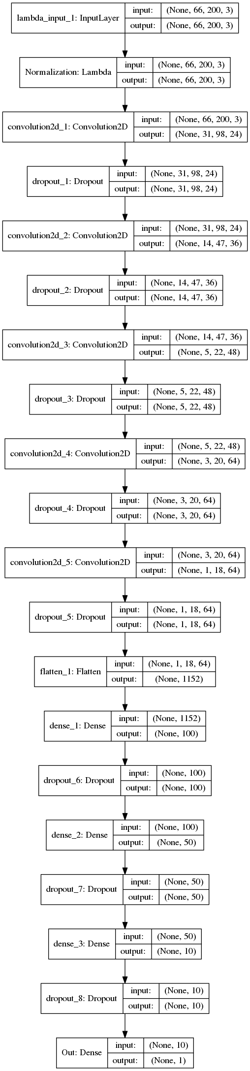
The model represented here is my implementation of the nvidia model mentioned previously. It is coded in python using keras (with tensor flow) in model.py and returned from the build_nvidia_model method. The complete project is on github here Udacity Behaviour Cloning Project
Input
The input is 66x200xC with C = 3 RGB color channels.
Architecture
Layer 0: Normalisation to range -1, 1 (1./127.5 -1)
Layer 1: Convolution with strides=(2,2), valid padding, kernel 5×5 and output shape 31x98x24, with elu activation and dropout
Layer 2: Convolution with strides=(2,2), valid padding, kernel 5×5 and output shape 14x47x36, with elu activation and dropout
Layer 3: Convolution with strides=(2,2), valid padding, kernel 5×5 and output shape 5x22x48, with elu activation and dropout
Layer 4: Convolution with strides=(1,1), valid padding, kernel 3×3 and output shape 3x20x64, with elu activation and dropout
Layer 5: Convolution with strides=(1,1), valid padding, kernel 3×3 and output shape 1x18x64, with elu activation and dropout
flatten 1152 output
Layer 6: Fully Connected with 100 outputs and dropout
Layer 7: Fully Connected with 50 outputs and dropout
Layer 8: Fully Connected with 10 outputs and dropout
dropout was set aggressively on each layer at .25 to avoid overtraining
Output
Layer Fully Connected with 1 output value for the steering angle.
The simulator captures data into a csv log file which references left, centre and right captured images within a sub directory. Telemetry data for steering, throttle, brake and speed is also contained in the log. Only steering was used in this project.
My initial investigation and analysis was performed in a Jupyter Notebook here.
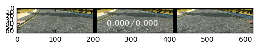
Before being fed into the model, the images are cropped to 66×200 starting at height 60 with width centered – A sample video of a run cropped.
Cropped left, centre and right camera image
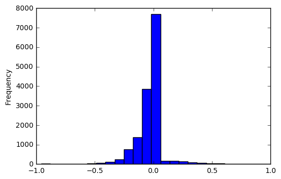
As seen in the following histogram a significant proportion of the data is for driving straight and its lopsided to left turns (being a negative steering angle is left) when using data generated following my conservative driving laps.
The log file was preprocessed to remove contiguous rows with a history of >5 records, with a 0.0 steering angle. This was the only preprocessing done outside of the batch generators used in training (random rows are augmented/jittered for each batch at model training time).
A left, centre or right camera was selected randomly for each row, with .25 angle ( for left and – for right) applied to the steering.
Jittering was applied per Vivek Yadav’s post to augment data. Images were randomly transformed in the x range by 100 pixels and in the y range by 10 pixels with 0.4 per xpixel adjusted against the steering angle. Brightness via a HSV (V channel) transform (.25 a random number in range 0 to 1) was also performed.
During batch generation, to compensate for the left turning, 50% of images were flipped (including reversing steering angle) if the absolute steering angle was > .1.
Finally images are cropped per above before being batched.
Model Training
Data was captured from the simulator. I drove conservatively around the track three times paying particular attention to the sharp right turn. I found connecting a PS3 controller allowed finer control then using the keyboard. At least once I waited till the last moment before taking the turn. This seems to have stopped the car ending up in the lake. Its also helped to overcome a symptom of the bias in the training data towards left turns. To further offset this risk, I validated the training using a test set I’d captured from the second track, which is a lot more windy.
Center camera has the steering angle and 1/r values displayed.
The Adam Optimizer was used with a mean squared error loss. A number of hyper-parameters were passed on the command line. The command I used looks such for a batch size of 500, 10 epochs (dropped out early if loss wasn’t improving), dropout at .25 with a training size of 50000 randomly augmented features with adjusted labels and 2000 random features & labels used for validation
To meet requirements, and hence pass the assignment, the vehicle has to drive around the first track staying on the road and not going up on the curb.
The model trained (which is saved), is used again in testing. The simulator feeds you the centre camera image, along with steering and throttle telemetry. In response you have to return the new steering angle and throttle values. I hard coded the throttle to .35. The image was cropped, the same as for training, then fed into the model for prediction giving the steering angle.
note: the trained model I used for the track 1 run, is different to the one used to run the simulator in track 2. I found that the data I originally used to train a model to run both tracks, would occasionally meander on track 1 quite wildly. Thus used training data to make it more conservative to meet requirements for the projects.


 which is then used as input into
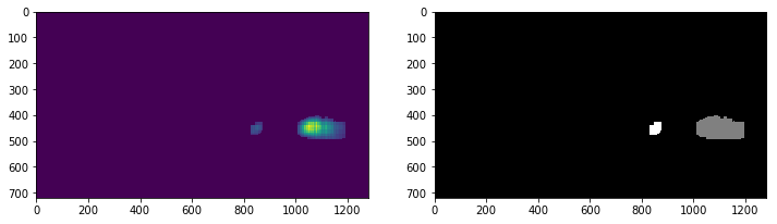


